Effective Area

This notebook builds off previously implementation inspections and will walk you through how to calculate effective areas for a given dataset. In this example, we will focus on using the DNNCascade dataset (https://wiki.icecube.wisc.edu/index.php/Cascade_Neutrino_Source_Dataset/Dataset_Performace). Additionally, the nuts and bolts that describe the actual mechanics of effective area calculations can be found in Brian Clark’s thesis (Section 5.3, pg 99 - https://etd.ohiolink.edu/apexprod/rws_etd/send_file/send?accession=osu1563461175725125&disposition=inline).

[82]:

#Libraries that will be used
import csky as cy
import histlite as hl
import matplotlib
import matplotlib.pyplot as plt
import numpy as np

cy.plotting.mrichman_mpl()

/home/mkovacevich/csky/csky/csky/plotting.py:92: MatplotlibDeprecationWarning: Support for setting the 'text.latex.preamble' or 'pgf.preamble' rcParam to a list of strings is deprecated since 3.3 and will be removed two minor releases later; set it to a single string instead.
  r'\SetSymbolFont{operators}   {sans}{OT1}{cmss} {m}{n}'

Loading the DNNCascade dataset into an analysis object below:

[83]:

repo = cy.selections.Repository()
specs = cy.selections.DNNCascadeDataSpecs.DNNC_10yr
ana = cy.get_analysis(repo, 'version-001-p01', specs)

Setting up Analysis for:
DNNCascade_10yr
Setting up DNNCascade_10yr...
Reading /data/ana/analyses/dnn_cascades/version-001-p01/MC_NuGen_bfrv1_2153x.npy ...
Reading /data/ana/analyses/dnn_cascades/version-001-p01/IC86_2011_exp.npy ...
Reading /data/ana/analyses/dnn_cascades/version-001-p01/IC86_2012_exp.npy ...
Reading /data/ana/analyses/dnn_cascades/version-001-p01/IC86_2013_exp.npy ...
Reading /data/ana/analyses/dnn_cascades/version-001-p01/IC86_2014_exp.npy ...
Reading /data/ana/analyses/dnn_cascades/version-001-p01/IC86_2015_exp.npy ...
Reading /data/ana/analyses/dnn_cascades/version-001-p01/IC86_2016_exp.npy ...
Reading /data/ana/analyses/dnn_cascades/version-001-p01/IC86_2017_exp.npy ...
Reading /data/ana/analyses/dnn_cascades/version-001-p01/IC86_2018_exp.npy ...
Reading /data/ana/analyses/dnn_cascades/version-001-p01/IC86_2019_exp.npy ...
Reading /data/ana/analyses/dnn_cascades/version-001-p01/IC86_2020_exp.npy ...
Reading /data/ana/analyses/dnn_cascades/version-001-p01/GRL/IC86_2011_exp.npy ...
Reading /data/ana/analyses/dnn_cascades/version-001-p01/GRL/IC86_2012_exp.npy ...
Reading /data/ana/analyses/dnn_cascades/version-001-p01/GRL/IC86_2013_exp.npy ...
Reading /data/ana/analyses/dnn_cascades/version-001-p01/GRL/IC86_2014_exp.npy ...
Reading /data/ana/analyses/dnn_cascades/version-001-p01/GRL/IC86_2015_exp.npy ...
Reading /data/ana/analyses/dnn_cascades/version-001-p01/GRL/IC86_2016_exp.npy ...
Reading /data/ana/analyses/dnn_cascades/version-001-p01/GRL/IC86_2017_exp.npy ...
Reading /data/ana/analyses/dnn_cascades/version-001-p01/GRL/IC86_2018_exp.npy ...
Reading /data/ana/analyses/dnn_cascades/version-001-p01/GRL/IC86_2019_exp.npy ...
Reading /data/ana/analyses/dnn_cascades/version-001-p01/GRL/IC86_2020_exp.npy ...
Energy PDF Ratio Model...
  * gamma = 4.0000 ...
Signal Acceptance Model...
  * gamma = 4.0000 ...
Done.

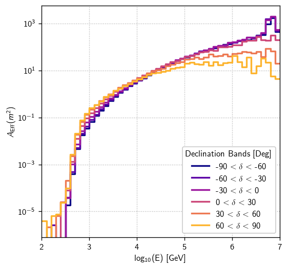
Now that we have loaded the dataset into an analysis object, we can calculate the Effective Area for different declinations. Since Effective Area is declination dependent, we look at different “declination bands” below - each band has a width of 30 degrees. This width was chosen to replicate the results that are shown in https://wiki.icecube.wisc.edu/index.php/File:Cascade_Neutrino_Source_Dataset_Effa.png (note the plotting differences). Below we have a function that we can walk through to calculate the Effective Areas. Note that we have to use oneweight and the MC True Energy to calculate the Effective Areas.

[84]:

def effective_area(dec_deg_min, dec_band_width, ana, ax, color, label='DNNC'):

    '''
    Note the following:

    *a=ana.anas[-1] may not contain the entire dataset. For tracks, it will only use the last season whereas DNNCascade
    loads as one season so the entire dataset is used.

    *dlogE is the logarithmic energy bin width

    *solid_angle represents the portion of the sky that we are observing with the detector

    *In the area eqn defined below, 1/ (1e4*np.log(10)) comes from eqn 5.12 in the thesis linked at the start
    of this notebook. The 1e4 accounts for converting from cm^2 -> m^2 and np.log(10) accounts for the ln(10) when
    differentiating dlog(E)
    '''

    dec_deg_max = dec_deg_min + dec_band_width
    a = ana.anas[-1]
    mask = (a.sig.dec < np.radians(dec_deg_max)) & (a.sig.dec > np.radians(dec_deg_min))

    dlogE=.1
    solid_angle=2*np.pi*(np.sin(np.radians(dec_deg_max))-np.sin(np.radians(dec_deg_min)))
    area= 1/ (1e4*np.log(10)) * (a.sig.oneweight[mask] / ( a.sig.true_energy[mask] *  solid_angle *  dlogE))

    bins=np.arange(2,7.01,.1)
    h = hl.hist(np.log10(a.sig.true_energy[mask]), weights=area, bins=bins);
    hl.plot1d(h, histtype='step', linewidth=2, color=color, label=rf'{dec_deg_min} $< \delta <$ {dec_deg_max}')

    ax.semilogy()
    ax.grid(True)
    ax.legend(loc='lower right', title=r'Declination Bands [Deg]')
    ax.set_ylabel('$A_\mathsf{Eff}$($m^2$)')
    ax.set_xlabel('log$_{10}$(E) [GeV]')
    ax.set_xlim((2,7))

    return h

[85]:

fig, ax = plt.subplots(1, 1, figsize=(5,5))

cmap = matplotlib.cm.get_cmap('plasma')
dec_band_width = 30
dec_deg_mins = np.arange(-90, 90, dec_band_width)

for idx, dec_deg_min in enumerate(dec_deg_mins):
    h = effective_area(dec_deg_min, dec_band_width, ana, ax, color=cmap(idx * (1/len(dec_deg_mins))))

[ ]: