Scaling up: analysis on a cluster

In this tutorial, we’ll offer some hints on how to scale up an analysis to a cluster-based workflow.

Introduction 

In previous tutorials, we’ve demonstrated how to perform various types of analysis using csky. However, all of these have been done the “quick and dirty” way. We haven’t explored how csky supports “high performance computing”, i.e. performing large batches of trials on a cluster.

Here we will be assuming that the user already knows how to perform individual tasks on their cluster(s) of choice, as well as how to work with scripts as opposed to notebooks more generally. The snippets found in this tutorial will be building blocks that can be assembled into per-task scripts, or separate commands within a single-script interface based on e.g. the click or fire modules. We take a conventional time-integrated all-sky scan as our testing scenario.

Setup 

Most scripts will start similarly to our other tutorial notebooks. Here we’ll set up some imports, and load up an Analysis. Since we aren’t actually going to use the cluster, we’ll keep the computational load down by working with just IC86-2011.

[1]:

# for cluster jobs, you may want to start by
# disabling interactive matplotlib graphics:
# import matplotlib
# matplotlib.use('Agg')

import numpy as np
import matplotlib.pyplot as plt
import os

import histlite as hl
import csky as cy

# set up timer
timer = cy.timing.Timer()
time = timer.time

# set up Analysis
ana_dir = cy.utils.ensure_dir('/data/user/mrichman/csky_cache/ana')
repo = cy.selections.repo
with time('ana setup'):
    ana = cy.get_analysis(repo, 'version-003-p02', cy.selections.PSDataSpecs.ps_2011, dir=ana_dir)
cy.CONF['ana'] = ana

Setting up Analysis for:
IC86_2011
Setting up IC86_2011...
Reading /data/ana/analyses/ps_tracks/version-003-p02/IC86_2011_MC.npy ...
Reading /data/ana/analyses/ps_tracks/version-003-p02/IC86_2011_exp.npy ...
Reading /data/ana/analyses/ps_tracks/version-003-p02/GRL/IC86_2011_exp.npy ...
<- /data/user/mrichman/csky_cache/ana/IC86_2011.subanalysis.version-003-p02.npy
Done.

0:00:01.503862 elapsed.

We will create a directory in which to store trials:

[2]:

trials_dir = cy.utils.ensure_dir('./trials/IC86_2011')

Since this tutorial is a notebook, we will make use of interactive plotting:

[3]:

%matplotlib inline

[4]:

cy.plotting.mrichman_mpl()

By the way: have a matplotlib configuration you’d like to share? Feel free to add it to plotting.py!

Finally, since we’re not distributing this tutorial’s calculations over a cluster, but rather will perform them sequentially on a cobalt, we will enable multiprocessing. For real cluster submissions, it’s best to split up the work in a way that does not rely on within-job multiprocessing.

[5]:

cy.CONF['mp_cpus'] = 10

Computing background trials 

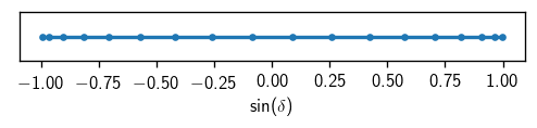
IceCube backgrounds are generally declination-dependent. Thus the first step towards an all-sky scan is to run background trials on a grid of declinations. A real analysis might space this grid in increments of 1° or 2°, but here we will use a 10° spacing just for demonstration.

[6]:

dec_degs = np.r_[-85:85.1:10]

[7]:

decs = np.radians(dec_degs)
sindecs = np.sin(decs)

The grid therefore looks as follows in \(\sin(\delta)\):

[8]:

fig, ax = plt.subplots(figsize=(5, .5))
ax.plot(sindecs, np.zeros_like(sindecs), '.-')
ax.set_yticks([])
ax.set_xlabel(r'$\sin(\delta)$');

Our function for computing background trials might look as follows:

[9]:

# we'll save, and later load, trials from this dir
bg_dir = cy.utils.ensure_dir('{}/bg'.format(trials_dir))

def do_background_trials(dec_deg, N=1000, seed=0):
    # get trial runner
    dec = np.radians(dec_deg)
    src = cy.sources(0, dec)
    tr = cy.get_trial_runner(src=src)
    # run trials
    trials = tr.get_many_fits(N, seed=seed, logging=False)
    # save to disk
    dir = cy.utils.ensure_dir('{}/dec/{:+04.0f}'.format(bg_dir, dec_deg))
    filename = '{}/trials__N_{:06d}_seed_{:04d}.npy'.format(dir, N, seed)
    print('->', filename)
    # notice: trials.as_array is a numpy structured array, not a cy.utils.Arrays
    np.save(filename, trials.as_array)

First we test this function out:

[10]:

do_background_trials(5)

-> ./trials/IC86_2011/bg/dec/+005/trials__N_001000_seed_0000.npy

It seems to work, so let’s clean up the test file and then do just enough trials to get a clue. This is where you want to submit cluster jobs to call do_background_trials!

[11]:

os.remove('./trials/IC86_2011/bg/dec/+005/trials__N_001000_seed_0000.npy')

[12]:

# just enough to demonstrate the data handling mechanisms we will be using
n_jobs = 2
N = 1000

# in real life you should keep track of compute time within your jobs
with time('bg trials'):
    for dec_deg in dec_degs:
        for seed in range(n_jobs):
            do_background_trials(dec_deg, N=N, seed=seed)

-> ./trials/IC86_2011/bg/dec/-085/trials__N_001000_seed_0000.npy
-> ./trials/IC86_2011/bg/dec/-085/trials__N_001000_seed_0001.npy
-> ./trials/IC86_2011/bg/dec/-075/trials__N_001000_seed_0000.npy
-> ./trials/IC86_2011/bg/dec/-075/trials__N_001000_seed_0001.npy
-> ./trials/IC86_2011/bg/dec/-065/trials__N_001000_seed_0000.npy
-> ./trials/IC86_2011/bg/dec/-065/trials__N_001000_seed_0001.npy
-> ./trials/IC86_2011/bg/dec/-055/trials__N_001000_seed_0000.npy
-> ./trials/IC86_2011/bg/dec/-055/trials__N_001000_seed_0001.npy
-> ./trials/IC86_2011/bg/dec/-045/trials__N_001000_seed_0000.npy
-> ./trials/IC86_2011/bg/dec/-045/trials__N_001000_seed_0001.npy
-> ./trials/IC86_2011/bg/dec/-035/trials__N_001000_seed_0000.npy
-> ./trials/IC86_2011/bg/dec/-035/trials__N_001000_seed_0001.npy
-> ./trials/IC86_2011/bg/dec/-025/trials__N_001000_seed_0000.npy
-> ./trials/IC86_2011/bg/dec/-025/trials__N_001000_seed_0001.npy
-> ./trials/IC86_2011/bg/dec/-015/trials__N_001000_seed_0000.npy
-> ./trials/IC86_2011/bg/dec/-015/trials__N_001000_seed_0001.npy
-> ./trials/IC86_2011/bg/dec/-005/trials__N_001000_seed_0000.npy
-> ./trials/IC86_2011/bg/dec/-005/trials__N_001000_seed_0001.npy
-> ./trials/IC86_2011/bg/dec/+005/trials__N_001000_seed_0000.npy
-> ./trials/IC86_2011/bg/dec/+005/trials__N_001000_seed_0001.npy
-> ./trials/IC86_2011/bg/dec/+015/trials__N_001000_seed_0000.npy
-> ./trials/IC86_2011/bg/dec/+015/trials__N_001000_seed_0001.npy
-> ./trials/IC86_2011/bg/dec/+025/trials__N_001000_seed_0000.npy
-> ./trials/IC86_2011/bg/dec/+025/trials__N_001000_seed_0001.npy
-> ./trials/IC86_2011/bg/dec/+035/trials__N_001000_seed_0000.npy
-> ./trials/IC86_2011/bg/dec/+035/trials__N_001000_seed_0001.npy
-> ./trials/IC86_2011/bg/dec/+045/trials__N_001000_seed_0000.npy
-> ./trials/IC86_2011/bg/dec/+045/trials__N_001000_seed_0001.npy
-> ./trials/IC86_2011/bg/dec/+055/trials__N_001000_seed_0000.npy
-> ./trials/IC86_2011/bg/dec/+055/trials__N_001000_seed_0001.npy
-> ./trials/IC86_2011/bg/dec/+065/trials__N_001000_seed_0000.npy
-> ./trials/IC86_2011/bg/dec/+065/trials__N_001000_seed_0001.npy
-> ./trials/IC86_2011/bg/dec/+075/trials__N_001000_seed_0000.npy
-> ./trials/IC86_2011/bg/dec/+075/trials__N_001000_seed_0001.npy
-> ./trials/IC86_2011/bg/dec/+085/trials__N_001000_seed_0000.npy
-> ./trials/IC86_2011/bg/dec/+085/trials__N_001000_seed_0001.npy

0:00:57.027624 elapsed.

Computing signal trials 

Signal trials are computed in similar fashion. However, now we want to keep track of the signal strength in addition to the declination.

[13]:

# we'll save, and later load, trials from this dir
sig_dir = cy.utils.ensure_dir('{}/sig'.format(trials_dir))

def do_signal_trials(dec_deg, n_sig, N=1000, seed=0):
    # get trial runner
    dec = np.radians(dec_deg)
    src = cy.sources(0, dec)
    tr = cy.get_trial_runner(src=src)
    # run trials
    trials = tr.get_many_fits(N, n_sig, poisson=True, seed=seed, logging=False)
    # save to disk
    dir = cy.utils.ensure_dir('{}/dec/{:+04.0f}/nsig/{:05.1f}'.format(sig_dir, dec_deg, n_sig))
    filename = '{}/trials__N_{:06d}_seed_{:04d}.npy'.format(dir, N, seed)
    print('->', filename)
    # notice: trials.as_array is a numpy structured array, not a cy.utils.Arrays
    np.save(filename, trials.as_array)

Once again, we start with a quick test:

[14]:

do_signal_trials(5, 10)

-> ./trials/IC86_2011/sig/dec/+005/nsig/010.0/trials__N_001000_seed_0000.npy

Then we clean up the test file and “submit” the “jobs”:

[15]:

os.remove('./trials/IC86_2011/sig/dec/+005/nsig/010.0/trials__N_001000_seed_0000.npy')

(skip ahead to working with background trials)

[16]:

# just enough to demonstrate the data handling mechanisms we will be using
N = 1000
n_jobs = 1
n_sigs = np.r_[2:10:2, 10:30.1:4]

with time('signal trials'):
    for dec_deg in dec_degs:
        for n_sig in n_sigs:
            for seed in range(n_jobs):
                do_signal_trials(dec_deg, n_sig, N=N, seed=seed)

-> ./trials/IC86_2011/sig/dec/-085/nsig/002.0/trials__N_001000_seed_0000.npy
-> ./trials/IC86_2011/sig/dec/-085/nsig/004.0/trials__N_001000_seed_0000.npy
-> ./trials/IC86_2011/sig/dec/-085/nsig/006.0/trials__N_001000_seed_0000.npy
-> ./trials/IC86_2011/sig/dec/-085/nsig/008.0/trials__N_001000_seed_0000.npy
-> ./trials/IC86_2011/sig/dec/-085/nsig/010.0/trials__N_001000_seed_0000.npy
-> ./trials/IC86_2011/sig/dec/-085/nsig/014.0/trials__N_001000_seed_0000.npy
-> ./trials/IC86_2011/sig/dec/-085/nsig/018.0/trials__N_001000_seed_0000.npy
-> ./trials/IC86_2011/sig/dec/-085/nsig/022.0/trials__N_001000_seed_0000.npy
-> ./trials/IC86_2011/sig/dec/-085/nsig/026.0/trials__N_001000_seed_0000.npy
-> ./trials/IC86_2011/sig/dec/-085/nsig/030.0/trials__N_001000_seed_0000.npy
-> ./trials/IC86_2011/sig/dec/-075/nsig/002.0/trials__N_001000_seed_0000.npy
-> ./trials/IC86_2011/sig/dec/-075/nsig/004.0/trials__N_001000_seed_0000.npy
-> ./trials/IC86_2011/sig/dec/-075/nsig/006.0/trials__N_001000_seed_0000.npy
-> ./trials/IC86_2011/sig/dec/-075/nsig/008.0/trials__N_001000_seed_0000.npy
-> ./trials/IC86_2011/sig/dec/-075/nsig/010.0/trials__N_001000_seed_0000.npy
-> ./trials/IC86_2011/sig/dec/-075/nsig/014.0/trials__N_001000_seed_0000.npy
-> ./trials/IC86_2011/sig/dec/-075/nsig/018.0/trials__N_001000_seed_0000.npy
-> ./trials/IC86_2011/sig/dec/-075/nsig/022.0/trials__N_001000_seed_0000.npy
-> ./trials/IC86_2011/sig/dec/-075/nsig/026.0/trials__N_001000_seed_0000.npy
-> ./trials/IC86_2011/sig/dec/-075/nsig/030.0/trials__N_001000_seed_0000.npy
-> ./trials/IC86_2011/sig/dec/-065/nsig/002.0/trials__N_001000_seed_0000.npy
-> ./trials/IC86_2011/sig/dec/-065/nsig/004.0/trials__N_001000_seed_0000.npy
-> ./trials/IC86_2011/sig/dec/-065/nsig/006.0/trials__N_001000_seed_0000.npy
-> ./trials/IC86_2011/sig/dec/-065/nsig/008.0/trials__N_001000_seed_0000.npy
-> ./trials/IC86_2011/sig/dec/-065/nsig/010.0/trials__N_001000_seed_0000.npy
-> ./trials/IC86_2011/sig/dec/-065/nsig/014.0/trials__N_001000_seed_0000.npy
-> ./trials/IC86_2011/sig/dec/-065/nsig/018.0/trials__N_001000_seed_0000.npy
-> ./trials/IC86_2011/sig/dec/-065/nsig/022.0/trials__N_001000_seed_0000.npy
-> ./trials/IC86_2011/sig/dec/-065/nsig/026.0/trials__N_001000_seed_0000.npy
-> ./trials/IC86_2011/sig/dec/-065/nsig/030.0/trials__N_001000_seed_0000.npy
-> ./trials/IC86_2011/sig/dec/-055/nsig/002.0/trials__N_001000_seed_0000.npy
-> ./trials/IC86_2011/sig/dec/-055/nsig/004.0/trials__N_001000_seed_0000.npy
-> ./trials/IC86_2011/sig/dec/-055/nsig/006.0/trials__N_001000_seed_0000.npy
-> ./trials/IC86_2011/sig/dec/-055/nsig/008.0/trials__N_001000_seed_0000.npy
-> ./trials/IC86_2011/sig/dec/-055/nsig/010.0/trials__N_001000_seed_0000.npy
-> ./trials/IC86_2011/sig/dec/-055/nsig/014.0/trials__N_001000_seed_0000.npy
-> ./trials/IC86_2011/sig/dec/-055/nsig/018.0/trials__N_001000_seed_0000.npy
-> ./trials/IC86_2011/sig/dec/-055/nsig/022.0/trials__N_001000_seed_0000.npy
-> ./trials/IC86_2011/sig/dec/-055/nsig/026.0/trials__N_001000_seed_0000.npy
-> ./trials/IC86_2011/sig/dec/-055/nsig/030.0/trials__N_001000_seed_0000.npy
-> ./trials/IC86_2011/sig/dec/-045/nsig/002.0/trials__N_001000_seed_0000.npy
-> ./trials/IC86_2011/sig/dec/-045/nsig/004.0/trials__N_001000_seed_0000.npy
-> ./trials/IC86_2011/sig/dec/-045/nsig/006.0/trials__N_001000_seed_0000.npy
-> ./trials/IC86_2011/sig/dec/-045/nsig/008.0/trials__N_001000_seed_0000.npy
-> ./trials/IC86_2011/sig/dec/-045/nsig/010.0/trials__N_001000_seed_0000.npy
-> ./trials/IC86_2011/sig/dec/-045/nsig/014.0/trials__N_001000_seed_0000.npy
-> ./trials/IC86_2011/sig/dec/-045/nsig/018.0/trials__N_001000_seed_0000.npy
-> ./trials/IC86_2011/sig/dec/-045/nsig/022.0/trials__N_001000_seed_0000.npy
-> ./trials/IC86_2011/sig/dec/-045/nsig/026.0/trials__N_001000_seed_0000.npy
-> ./trials/IC86_2011/sig/dec/-045/nsig/030.0/trials__N_001000_seed_0000.npy
-> ./trials/IC86_2011/sig/dec/-035/nsig/002.0/trials__N_001000_seed_0000.npy
-> ./trials/IC86_2011/sig/dec/-035/nsig/004.0/trials__N_001000_seed_0000.npy
-> ./trials/IC86_2011/sig/dec/-035/nsig/006.0/trials__N_001000_seed_0000.npy
-> ./trials/IC86_2011/sig/dec/-035/nsig/008.0/trials__N_001000_seed_0000.npy
-> ./trials/IC86_2011/sig/dec/-035/nsig/010.0/trials__N_001000_seed_0000.npy
-> ./trials/IC86_2011/sig/dec/-035/nsig/014.0/trials__N_001000_seed_0000.npy
-> ./trials/IC86_2011/sig/dec/-035/nsig/018.0/trials__N_001000_seed_0000.npy
-> ./trials/IC86_2011/sig/dec/-035/nsig/022.0/trials__N_001000_seed_0000.npy
-> ./trials/IC86_2011/sig/dec/-035/nsig/026.0/trials__N_001000_seed_0000.npy
-> ./trials/IC86_2011/sig/dec/-035/nsig/030.0/trials__N_001000_seed_0000.npy
-> ./trials/IC86_2011/sig/dec/-025/nsig/002.0/trials__N_001000_seed_0000.npy
-> ./trials/IC86_2011/sig/dec/-025/nsig/004.0/trials__N_001000_seed_0000.npy
-> ./trials/IC86_2011/sig/dec/-025/nsig/006.0/trials__N_001000_seed_0000.npy
-> ./trials/IC86_2011/sig/dec/-025/nsig/008.0/trials__N_001000_seed_0000.npy
-> ./trials/IC86_2011/sig/dec/-025/nsig/010.0/trials__N_001000_seed_0000.npy
-> ./trials/IC86_2011/sig/dec/-025/nsig/014.0/trials__N_001000_seed_0000.npy
-> ./trials/IC86_2011/sig/dec/-025/nsig/018.0/trials__N_001000_seed_0000.npy
-> ./trials/IC86_2011/sig/dec/-025/nsig/022.0/trials__N_001000_seed_0000.npy
-> ./trials/IC86_2011/sig/dec/-025/nsig/026.0/trials__N_001000_seed_0000.npy
-> ./trials/IC86_2011/sig/dec/-025/nsig/030.0/trials__N_001000_seed_0000.npy
-> ./trials/IC86_2011/sig/dec/-015/nsig/002.0/trials__N_001000_seed_0000.npy
-> ./trials/IC86_2011/sig/dec/-015/nsig/004.0/trials__N_001000_seed_0000.npy
-> ./trials/IC86_2011/sig/dec/-015/nsig/006.0/trials__N_001000_seed_0000.npy
-> ./trials/IC86_2011/sig/dec/-015/nsig/008.0/trials__N_001000_seed_0000.npy
-> ./trials/IC86_2011/sig/dec/-015/nsig/010.0/trials__N_001000_seed_0000.npy
-> ./trials/IC86_2011/sig/dec/-015/nsig/014.0/trials__N_001000_seed_0000.npy
-> ./trials/IC86_2011/sig/dec/-015/nsig/018.0/trials__N_001000_seed_0000.npy
-> ./trials/IC86_2011/sig/dec/-015/nsig/022.0/trials__N_001000_seed_0000.npy
-> ./trials/IC86_2011/sig/dec/-015/nsig/026.0/trials__N_001000_seed_0000.npy
-> ./trials/IC86_2011/sig/dec/-015/nsig/030.0/trials__N_001000_seed_0000.npy
-> ./trials/IC86_2011/sig/dec/-005/nsig/002.0/trials__N_001000_seed_0000.npy
-> ./trials/IC86_2011/sig/dec/-005/nsig/004.0/trials__N_001000_seed_0000.npy
-> ./trials/IC86_2011/sig/dec/-005/nsig/006.0/trials__N_001000_seed_0000.npy
-> ./trials/IC86_2011/sig/dec/-005/nsig/008.0/trials__N_001000_seed_0000.npy
-> ./trials/IC86_2011/sig/dec/-005/nsig/010.0/trials__N_001000_seed_0000.npy
-> ./trials/IC86_2011/sig/dec/-005/nsig/014.0/trials__N_001000_seed_0000.npy
-> ./trials/IC86_2011/sig/dec/-005/nsig/018.0/trials__N_001000_seed_0000.npy
-> ./trials/IC86_2011/sig/dec/-005/nsig/022.0/trials__N_001000_seed_0000.npy
-> ./trials/IC86_2011/sig/dec/-005/nsig/026.0/trials__N_001000_seed_0000.npy
-> ./trials/IC86_2011/sig/dec/-005/nsig/030.0/trials__N_001000_seed_0000.npy
-> ./trials/IC86_2011/sig/dec/+005/nsig/002.0/trials__N_001000_seed_0000.npy
-> ./trials/IC86_2011/sig/dec/+005/nsig/004.0/trials__N_001000_seed_0000.npy
-> ./trials/IC86_2011/sig/dec/+005/nsig/006.0/trials__N_001000_seed_0000.npy
-> ./trials/IC86_2011/sig/dec/+005/nsig/008.0/trials__N_001000_seed_0000.npy
-> ./trials/IC86_2011/sig/dec/+005/nsig/010.0/trials__N_001000_seed_0000.npy
-> ./trials/IC86_2011/sig/dec/+005/nsig/014.0/trials__N_001000_seed_0000.npy
-> ./trials/IC86_2011/sig/dec/+005/nsig/018.0/trials__N_001000_seed_0000.npy
-> ./trials/IC86_2011/sig/dec/+005/nsig/022.0/trials__N_001000_seed_0000.npy
-> ./trials/IC86_2011/sig/dec/+005/nsig/026.0/trials__N_001000_seed_0000.npy
-> ./trials/IC86_2011/sig/dec/+005/nsig/030.0/trials__N_001000_seed_0000.npy
-> ./trials/IC86_2011/sig/dec/+015/nsig/002.0/trials__N_001000_seed_0000.npy
-> ./trials/IC86_2011/sig/dec/+015/nsig/004.0/trials__N_001000_seed_0000.npy
-> ./trials/IC86_2011/sig/dec/+015/nsig/006.0/trials__N_001000_seed_0000.npy
-> ./trials/IC86_2011/sig/dec/+015/nsig/008.0/trials__N_001000_seed_0000.npy
-> ./trials/IC86_2011/sig/dec/+015/nsig/010.0/trials__N_001000_seed_0000.npy
-> ./trials/IC86_2011/sig/dec/+015/nsig/014.0/trials__N_001000_seed_0000.npy
-> ./trials/IC86_2011/sig/dec/+015/nsig/018.0/trials__N_001000_seed_0000.npy
-> ./trials/IC86_2011/sig/dec/+015/nsig/022.0/trials__N_001000_seed_0000.npy
-> ./trials/IC86_2011/sig/dec/+015/nsig/026.0/trials__N_001000_seed_0000.npy
-> ./trials/IC86_2011/sig/dec/+015/nsig/030.0/trials__N_001000_seed_0000.npy
-> ./trials/IC86_2011/sig/dec/+025/nsig/002.0/trials__N_001000_seed_0000.npy
-> ./trials/IC86_2011/sig/dec/+025/nsig/004.0/trials__N_001000_seed_0000.npy
-> ./trials/IC86_2011/sig/dec/+025/nsig/006.0/trials__N_001000_seed_0000.npy
-> ./trials/IC86_2011/sig/dec/+025/nsig/008.0/trials__N_001000_seed_0000.npy
-> ./trials/IC86_2011/sig/dec/+025/nsig/010.0/trials__N_001000_seed_0000.npy
-> ./trials/IC86_2011/sig/dec/+025/nsig/014.0/trials__N_001000_seed_0000.npy
-> ./trials/IC86_2011/sig/dec/+025/nsig/018.0/trials__N_001000_seed_0000.npy
-> ./trials/IC86_2011/sig/dec/+025/nsig/022.0/trials__N_001000_seed_0000.npy
-> ./trials/IC86_2011/sig/dec/+025/nsig/026.0/trials__N_001000_seed_0000.npy
-> ./trials/IC86_2011/sig/dec/+025/nsig/030.0/trials__N_001000_seed_0000.npy
-> ./trials/IC86_2011/sig/dec/+035/nsig/002.0/trials__N_001000_seed_0000.npy
-> ./trials/IC86_2011/sig/dec/+035/nsig/004.0/trials__N_001000_seed_0000.npy
-> ./trials/IC86_2011/sig/dec/+035/nsig/006.0/trials__N_001000_seed_0000.npy
-> ./trials/IC86_2011/sig/dec/+035/nsig/008.0/trials__N_001000_seed_0000.npy
-> ./trials/IC86_2011/sig/dec/+035/nsig/010.0/trials__N_001000_seed_0000.npy
-> ./trials/IC86_2011/sig/dec/+035/nsig/014.0/trials__N_001000_seed_0000.npy
-> ./trials/IC86_2011/sig/dec/+035/nsig/018.0/trials__N_001000_seed_0000.npy
-> ./trials/IC86_2011/sig/dec/+035/nsig/022.0/trials__N_001000_seed_0000.npy
-> ./trials/IC86_2011/sig/dec/+035/nsig/026.0/trials__N_001000_seed_0000.npy
-> ./trials/IC86_2011/sig/dec/+035/nsig/030.0/trials__N_001000_seed_0000.npy
-> ./trials/IC86_2011/sig/dec/+045/nsig/002.0/trials__N_001000_seed_0000.npy
-> ./trials/IC86_2011/sig/dec/+045/nsig/004.0/trials__N_001000_seed_0000.npy
-> ./trials/IC86_2011/sig/dec/+045/nsig/006.0/trials__N_001000_seed_0000.npy
-> ./trials/IC86_2011/sig/dec/+045/nsig/008.0/trials__N_001000_seed_0000.npy
-> ./trials/IC86_2011/sig/dec/+045/nsig/010.0/trials__N_001000_seed_0000.npy
-> ./trials/IC86_2011/sig/dec/+045/nsig/014.0/trials__N_001000_seed_0000.npy
-> ./trials/IC86_2011/sig/dec/+045/nsig/018.0/trials__N_001000_seed_0000.npy
-> ./trials/IC86_2011/sig/dec/+045/nsig/022.0/trials__N_001000_seed_0000.npy
-> ./trials/IC86_2011/sig/dec/+045/nsig/026.0/trials__N_001000_seed_0000.npy
-> ./trials/IC86_2011/sig/dec/+045/nsig/030.0/trials__N_001000_seed_0000.npy
-> ./trials/IC86_2011/sig/dec/+055/nsig/002.0/trials__N_001000_seed_0000.npy
-> ./trials/IC86_2011/sig/dec/+055/nsig/004.0/trials__N_001000_seed_0000.npy
-> ./trials/IC86_2011/sig/dec/+055/nsig/006.0/trials__N_001000_seed_0000.npy
-> ./trials/IC86_2011/sig/dec/+055/nsig/008.0/trials__N_001000_seed_0000.npy
-> ./trials/IC86_2011/sig/dec/+055/nsig/010.0/trials__N_001000_seed_0000.npy
-> ./trials/IC86_2011/sig/dec/+055/nsig/014.0/trials__N_001000_seed_0000.npy
-> ./trials/IC86_2011/sig/dec/+055/nsig/018.0/trials__N_001000_seed_0000.npy
-> ./trials/IC86_2011/sig/dec/+055/nsig/022.0/trials__N_001000_seed_0000.npy
-> ./trials/IC86_2011/sig/dec/+055/nsig/026.0/trials__N_001000_seed_0000.npy
-> ./trials/IC86_2011/sig/dec/+055/nsig/030.0/trials__N_001000_seed_0000.npy
-> ./trials/IC86_2011/sig/dec/+065/nsig/002.0/trials__N_001000_seed_0000.npy
-> ./trials/IC86_2011/sig/dec/+065/nsig/004.0/trials__N_001000_seed_0000.npy
-> ./trials/IC86_2011/sig/dec/+065/nsig/006.0/trials__N_001000_seed_0000.npy
-> ./trials/IC86_2011/sig/dec/+065/nsig/008.0/trials__N_001000_seed_0000.npy
-> ./trials/IC86_2011/sig/dec/+065/nsig/010.0/trials__N_001000_seed_0000.npy
-> ./trials/IC86_2011/sig/dec/+065/nsig/014.0/trials__N_001000_seed_0000.npy
-> ./trials/IC86_2011/sig/dec/+065/nsig/018.0/trials__N_001000_seed_0000.npy
-> ./trials/IC86_2011/sig/dec/+065/nsig/022.0/trials__N_001000_seed_0000.npy
-> ./trials/IC86_2011/sig/dec/+065/nsig/026.0/trials__N_001000_seed_0000.npy
-> ./trials/IC86_2011/sig/dec/+065/nsig/030.0/trials__N_001000_seed_0000.npy
-> ./trials/IC86_2011/sig/dec/+075/nsig/002.0/trials__N_001000_seed_0000.npy
-> ./trials/IC86_2011/sig/dec/+075/nsig/004.0/trials__N_001000_seed_0000.npy
-> ./trials/IC86_2011/sig/dec/+075/nsig/006.0/trials__N_001000_seed_0000.npy
-> ./trials/IC86_2011/sig/dec/+075/nsig/008.0/trials__N_001000_seed_0000.npy
-> ./trials/IC86_2011/sig/dec/+075/nsig/010.0/trials__N_001000_seed_0000.npy
-> ./trials/IC86_2011/sig/dec/+075/nsig/014.0/trials__N_001000_seed_0000.npy
-> ./trials/IC86_2011/sig/dec/+075/nsig/018.0/trials__N_001000_seed_0000.npy
-> ./trials/IC86_2011/sig/dec/+075/nsig/022.0/trials__N_001000_seed_0000.npy
-> ./trials/IC86_2011/sig/dec/+075/nsig/026.0/trials__N_001000_seed_0000.npy
-> ./trials/IC86_2011/sig/dec/+075/nsig/030.0/trials__N_001000_seed_0000.npy
-> ./trials/IC86_2011/sig/dec/+085/nsig/002.0/trials__N_001000_seed_0000.npy
-> ./trials/IC86_2011/sig/dec/+085/nsig/004.0/trials__N_001000_seed_0000.npy
-> ./trials/IC86_2011/sig/dec/+085/nsig/006.0/trials__N_001000_seed_0000.npy
-> ./trials/IC86_2011/sig/dec/+085/nsig/008.0/trials__N_001000_seed_0000.npy
-> ./trials/IC86_2011/sig/dec/+085/nsig/010.0/trials__N_001000_seed_0000.npy
-> ./trials/IC86_2011/sig/dec/+085/nsig/014.0/trials__N_001000_seed_0000.npy
-> ./trials/IC86_2011/sig/dec/+085/nsig/018.0/trials__N_001000_seed_0000.npy
-> ./trials/IC86_2011/sig/dec/+085/nsig/022.0/trials__N_001000_seed_0000.npy
-> ./trials/IC86_2011/sig/dec/+085/nsig/026.0/trials__N_001000_seed_0000.npy
-> ./trials/IC86_2011/sig/dec/+085/nsig/030.0/trials__N_001000_seed_0000.npy

0:07:15.878014 elapsed.

Working with background trials 

Now that our trials are on disk, we can load them up to inspect the background properties and to compute the sensitivity and discovery potential. First, you should confirm in your shell that the saved files look as expected. Here we’ll pipe through head but in real life you might want to pipe through less or vim -R - instead.

[17]:

!find trials/IC86_2011/bg | sort | head -n20

trials/IC86_2011/bg
trials/IC86_2011/bg/dec
trials/IC86_2011/bg/dec/-005
trials/IC86_2011/bg/dec/+005
trials/IC86_2011/bg/dec/-005/trials__N_001000_seed_0000.npy
trials/IC86_2011/bg/dec/+005/trials__N_001000_seed_0000.npy
trials/IC86_2011/bg/dec/-005/trials__N_001000_seed_0001.npy
trials/IC86_2011/bg/dec/+005/trials__N_001000_seed_0001.npy
trials/IC86_2011/bg/dec/-015
trials/IC86_2011/bg/dec/+015
trials/IC86_2011/bg/dec/-015/trials__N_001000_seed_0000.npy
trials/IC86_2011/bg/dec/+015/trials__N_001000_seed_0000.npy
trials/IC86_2011/bg/dec/-015/trials__N_001000_seed_0001.npy
trials/IC86_2011/bg/dec/+015/trials__N_001000_seed_0001.npy
trials/IC86_2011/bg/dec/-025
trials/IC86_2011/bg/dec/+025
trials/IC86_2011/bg/dec/-025/trials__N_001000_seed_0000.npy
trials/IC86_2011/bg/dec/+025/trials__N_001000_seed_0000.npy
trials/IC86_2011/bg/dec/-025/trials__N_001000_seed_0001.npy
trials/IC86_2011/bg/dec/+025/trials__N_001000_seed_0001.npy

csky provides the cy.bk module for book keeping. First let’s load the background trials:

[18]:

def ndarray_to_Chi2TSD(trials):
    return cy.dists.Chi2TSD(cy.utils.Arrays(trials))

[19]:

with time('load bg trials'):
    bg = cy.bk.get_all(
        # disk location
        '{}/dec'.format(bg_dir),
        # filename pattern
        'trials*npy',
        # how to combine items within each directory
        merge=np.concatenate,
        # what to do with items after merge
        post_convert=ndarray_to_Chi2TSD)

36 files loaded.

0:00:02.611293 elapsed.

The result is that now bg is a dict containing the background distributions for each declination:

[20]:

bg

[20]:

{5: Chi2TSD(2000 trials, eta=0.582, ndof=1.038, median=0.041 (from fit 0.046)),
 15: Chi2TSD(2000 trials, eta=0.602, ndof=1.116, median=0.086 (from fit 0.077)),
 25: Chi2TSD(2000 trials, eta=0.601, ndof=1.074, median=0.070 (from fit 0.066)),
 35: Chi2TSD(2000 trials, eta=0.514, ndof=1.118, median=0.003 (from fit 0.003)),
 45: Chi2TSD(2000 trials, eta=0.498, ndof=1.037, median=0.000 (from fit 0.000)),
 55: Chi2TSD(2000 trials, eta=0.498, ndof=1.071, median=0.000 (from fit 0.000)),
 65: Chi2TSD(2000 trials, eta=0.593, ndof=0.990, median=0.059 (from fit 0.059)),
 75: Chi2TSD(2000 trials, eta=0.384, ndof=1.043, median=0.000 (from fit 0.000)),
 85: Chi2TSD(2000 trials, eta=0.298, ndof=0.721, median=0.000 (from fit 0.000)),
 -5: Chi2TSD(2000 trials, eta=0.492, ndof=1.085, median=0.000 (from fit 0.000)),
 -15: Chi2TSD(2000 trials, eta=0.450, ndof=1.123, median=0.000 (from fit 0.000)),
 -25: Chi2TSD(2000 trials, eta=0.514, ndof=1.058, median=0.002 (from fit 0.002)),
 -35: Chi2TSD(2000 trials, eta=0.472, ndof=1.090, median=0.000 (from fit 0.000)),
 -45: Chi2TSD(2000 trials, eta=0.513, ndof=0.996, median=0.001 (from fit 0.001)),
 -55: Chi2TSD(2000 trials, eta=0.532, ndof=1.238, median=0.017 (from fit 0.018)),
 -65: Chi2TSD(2000 trials, eta=0.537, ndof=1.138, median=0.016 (from fit 0.015)),
 -75: Chi2TSD(2000 trials, eta=0.537, ndof=1.094, median=0.011 (from fit 0.014)),
 -85: Chi2TSD(2000 trials, eta=0.240, ndof=0.896, median=0.000 (from fit 0.000))}

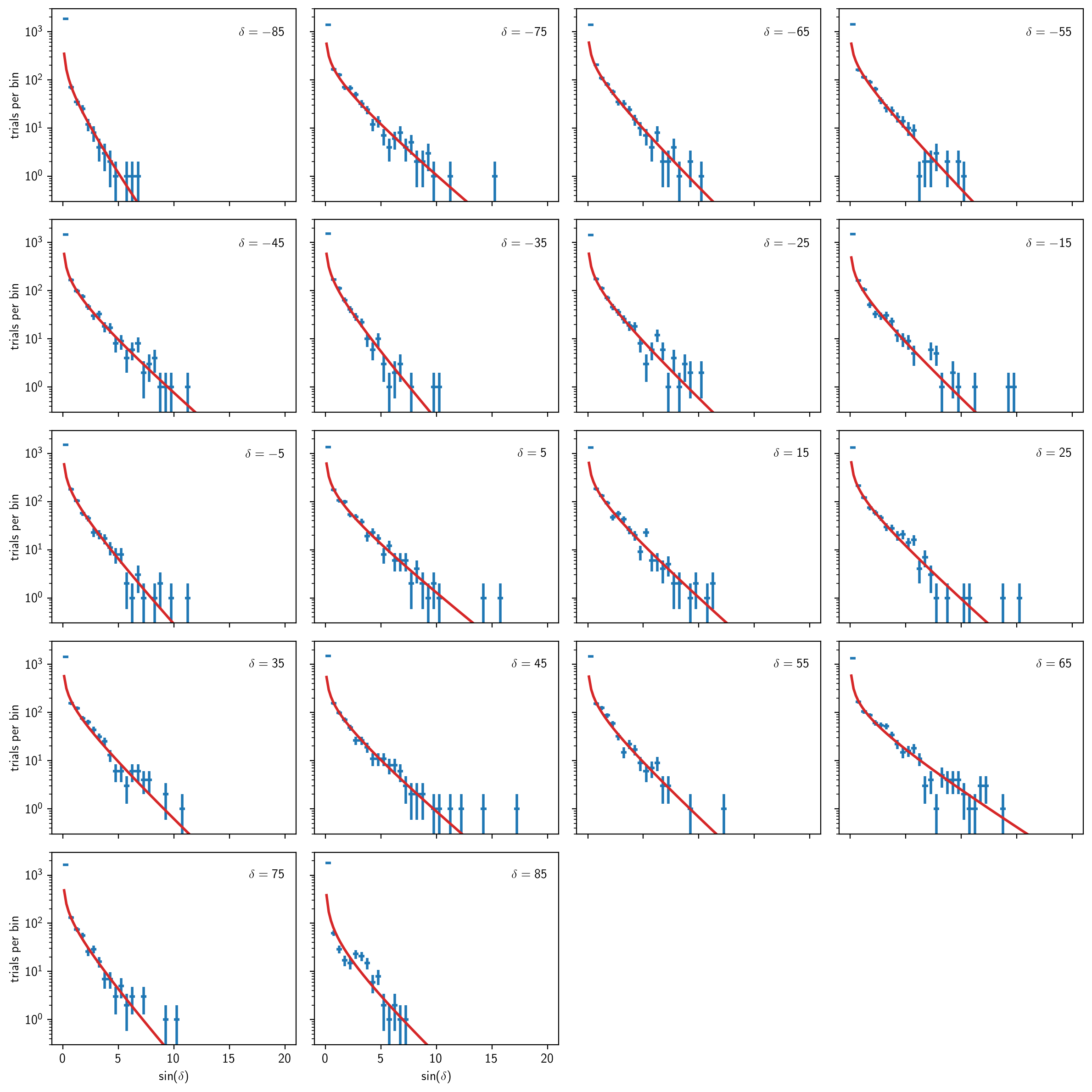
We can plot all of these out on a big grid:

[21]:

# just choose enough nrow x ncol to fit the whole grid
nrow, ncol = 5, 4
fig, aaxs = plt.subplots(nrow, ncol, figsize=(12,12), sharex=True, sharey=True, dpi=200)
axs = np.ravel(aaxs)
# keep track of which ax's we already used
used_axs = []
for (i, dec_deg) in enumerate(dec_degs):
    ax = axs[i]
    # plot histogram
    b = bg[dec_deg]
    h = b.get_hist(bins=40, range=(0, 20))
    hl.plot1d(ax, h, crosses=True)
    # plot chi2 fit to nonzero values
    norm = h.integrate().values
    ts = np.linspace(.1, h.range[0][1], 100)
    ax.plot(ts, norm * b.pdf(ts))
    # set limits and label dec
    ax.semilogy(nonposy='clip')
    ax.set_ylim(.3, 3e3)
    ax.text(20, 1e3, r'$\delta={:.0f}$'.format(dec_deg), ha='right', va='center')
    used_axs.append(ax)
# hide unused ax's
for ax in axs:
    if ax not in used_axs:
        ax.set_visible(False)
# add x and y labels
for ax in aaxs[-1]:
    if ax in used_axs:
        ax.set_xlabel(r'$\sin(\delta)$')
for ax in aaxs[:,0]:
    ax.set_ylabel(r'trials per bin')
plt.tight_layout()

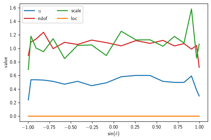
We can also plot a summary of the \(\chi^2\) fit parameters:

[22]:

etas = np.array([bg[d].eta for d in dec_degs])
ndofs = np.array([bg[d].ndof for d in dec_degs])
locs = np.array([bg[d].loc for d in dec_degs])
scales = np.array([bg[d].scale for d in dec_degs])

[23]:

fig, ax = plt.subplots()
ax.plot(sindecs, etas, label=r'$\eta$')
ax.plot(sindecs, ndofs, label='ndof')
ax.plot(sindecs, scales, label='scale')
ax.plot(sindecs, locs, label='loc')
ax.legend(ncol=2)
ax.set_xlabel(r'$\sin(\delta)$')
ax.set_ylabel(r'value')
plt.tight_layout()

At this point in a real analysis, you will want to decide whether to go back and perform more trials at these or additional declinations. While the \(\chi^2\) fits above are generally decent, we haven’t really done enough trials to pin down the discovery potential accurately (or perhaps even the sensitivity).

Since this is just a tutorial, we press on.

Working with signal trials: sensitivity and discovery potential 

We briefly check the signal trial structure on disk:

[24]:

!find trials/IC86_2011/sig | sort | head -n20

trials/IC86_2011/sig
trials/IC86_2011/sig/dec
trials/IC86_2011/sig/dec/-005
trials/IC86_2011/sig/dec/+005
trials/IC86_2011/sig/dec/-005/nsig
trials/IC86_2011/sig/dec/+005/nsig
trials/IC86_2011/sig/dec/-005/nsig/002.0
trials/IC86_2011/sig/dec/+005/nsig/002.0
trials/IC86_2011/sig/dec/-005/nsig/002.0/trials__N_001000_seed_0000.npy
trials/IC86_2011/sig/dec/+005/nsig/002.0/trials__N_001000_seed_0000.npy
trials/IC86_2011/sig/dec/-005/nsig/004.0
trials/IC86_2011/sig/dec/+005/nsig/004.0
trials/IC86_2011/sig/dec/-005/nsig/004.0/trials__N_001000_seed_0000.npy
trials/IC86_2011/sig/dec/+005/nsig/004.0/trials__N_001000_seed_0000.npy
trials/IC86_2011/sig/dec/-005/nsig/006.0
trials/IC86_2011/sig/dec/+005/nsig/006.0
trials/IC86_2011/sig/dec/-005/nsig/006.0/trials__N_001000_seed_0000.npy
trials/IC86_2011/sig/dec/+005/nsig/006.0/trials__N_001000_seed_0000.npy
trials/IC86_2011/sig/dec/-005/nsig/008.0
trials/IC86_2011/sig/dec/+005/nsig/008.0
sort: write failed: standard output: Broken pipe
sort: write error

We load the signal trials in similar fashion:

[25]:

with time('load sig trials'):
    sig = cy.bk.get_all(sig_dir, 'trials*npy', merge=np.concatenate, post_convert=cy.utils.Arrays)

180 files loaded.

0:00:00.832596 elapsed.

Now we have a deeply nested dict. To get to one specific batch of trials, we need to descend through the layers:

[26]:

sig['dec'][5]['nsig'][10]

[26]:

Arrays(1000 items | columns: gamma, ns, ts)

csky provides a function for doing this conveniently, including fuzzy matching for numerical values:

[27]:

cy.bk.get_best(sig, 'dec', 5, 'nsig', 10)

[27]:

Arrays(1000 items | columns: gamma, ns, ts)

You don’t need to descend all the way to the end of the tree:

[28]:

cy.bk.get_best(sig, 'dec', 5, 'nsig')

[28]:

{2.0: Arrays(1000 items | columns: gamma, ns, ts),
 4.0: Arrays(1000 items | columns: gamma, ns, ts),
 6.0: Arrays(1000 items | columns: gamma, ns, ts),
 8.0: Arrays(1000 items | columns: gamma, ns, ts),
 10.0: Arrays(1000 items | columns: gamma, ns, ts),
 14.0: Arrays(1000 items | columns: gamma, ns, ts),
 18.0: Arrays(1000 items | columns: gamma, ns, ts),
 22.0: Arrays(1000 items | columns: gamma, ns, ts),
 26.0: Arrays(1000 items | columns: gamma, ns, ts),
 30.0: Arrays(1000 items | columns: gamma, ns, ts)}

Maybe now the motivation for including the extra dec and nsig levels becomes clear: it makes it explicit, both on disk and in the in-memory data structure, what each level actually means.

We can use dicts of this form to compute sensitivity and discovery potential fluxes. But first, let’s get another dict of per-dec trial runners:

[29]:

with time('setup trial runners for sens/disc'):
    trs = {d: cy.get_trial_runner(src=cy.sources(0, d, deg=True)) for d in dec_degs}


0:00:01.046077 elapsed.

Then we define a little helper function:

[30]:

@np.vectorize
def find_n_sig(dec_deg, beta=0.9, nsigma=None):
    # get signal trials, background distribution, and trial runner
    sig_trials = cy.bk.get_best(sig, 'dec', dec_deg, 'nsig')
    b = cy.bk.get_best(bg, dec_deg)
    tr = cy.bk.get_best(trs, dec_deg)
    # determine ts threshold
    if nsigma is not None:
        ts = b.isf_nsigma(nsigma)
    else:
        ts = b.median()
    # include background trials in calculation
    trials = {0: b.trials}
    trials.update(sig_trials)
    # get number of signal events
    # (arguments prevent additional trials from being run)
    result = tr.find_n_sig(ts, beta, max_batch_size=0, logging=False, trials=trials, n_bootstrap=1)
    # return flux
    return tr.to_E2dNdE(result, E0=100, unit=1e3)

In your own analysis, you might define a slightly different helper function with options to return the number of events or the relative error rather than the flux; options to choose different E0 and/or unit; or options to consider different scenarios you may have computed such as different spectral indices, spectral cutoffs, source extensions, etc.

Now we call the function to compute the sensitivity and discovery potential on our grid of declinations:

[31]:

with time('compute sensitivity'):
    fluxs_sens = find_n_sig(dec_degs)
with time('compute discovery potential'):
    fluxs_disc = find_n_sig(dec_degs, beta=0.5, nsigma=5)


0:00:01.763108 elapsed.

0:00:01.817958 elapsed.

Finally, we make the plot:

[32]:

fig, ax = plt.subplots()
# '.-' dot-plus-line style not attractive, but useful for early-stage plotting
ax.semilogy(sindecs, fluxs_disc, '.-', color='C1', label=r'Discovery Potential ($5\sigma$)')
ax.semilogy(sindecs, fluxs_sens, '.-', color='C0', label=r'Sensitivity')
ax.set_xlabel(r'$\sin(\delta)$')
ax.set_ylabel(r'$E^2\cdot dN/dE\ \ [\text{TeV}\,\text{cm}^{-2}\,\text{s}]$')
ax.legend()
ax.grid()
plt.tight_layout()

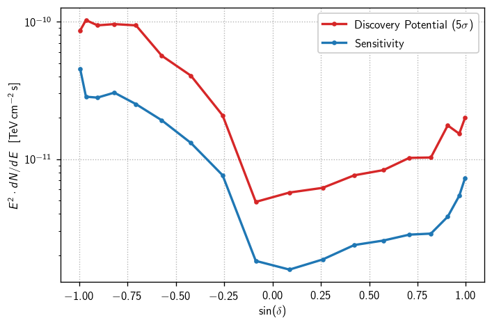
In real life, this is a moment for solemn contemplation. What does this plot tell us?

Is the declination dependence as expected for this selection? (yes) (approximately)
Are these values in the expected regime? (yes)
In particular, does this compare/contrast as expected with precedent? (yes) (see IC86-2011 plots)
Did we do enough background trials? (no) (visible fluctuations, possibly under-estimated discovery potential)
Is our declination grid sufficiently dense? (no) (behavior not well resolved near equator)

Before pressing ahead with an all-sky scan, the answers to all of these should be “yes”.

Since this is just a tutorial, we press on.

All-sky scan: p-values 

csky provides SkyScanTrialRunner for performing all-sky scans. To unblind one properly, we need not just a map of TS over the whole sky, but the corresponding p-values based on declination-dependent background distributions. Specifically, SkyScanTrialRunner accepts an argument ts_to_p=func, where it is expected that func(dec_in_radians, ts) -> p.

In general, a proper all-sky scan is performed on a healpix grid with pixels that are small compared to the angular resolution. Thus the scan grid should be dense compared to the required background distribution calculation grid. However, this means that you need to decide how to interpolate between declinations.

csky offers one possible solution: cy.dists.ts_to_p(). We define a trivial wrapper:

[33]:

def ts_to_p(dec, ts):
    # our background characterization was done on a grid of dec in degrees
    key = np.degrees(dec)
    # find and return the result
    return cy.dists.ts_to_p(bg, key, ts)

For example, consider a couple of arbitrary declinations and possible TS values:

[34]:

ts_to_p(np.array([np.pi/4, -np.pi/4]),
        np.array([10, .01]))

[34]:

array([0.00189439, 0.47481927])

What is cy.dists.ts_to_p doing behind the scenes? For any given declination, it finds the nearest smaller and larger background distribution declinations and computes p-values based on each one. Then it linearly interpolates — if the given declination is closer to the nearest smaller distribution, the final p-value will be closer to the one obtained from that distribution. Of course, if a given declination is beyond the smallest or largest background distribution declination, then that endpoint distribution alone is used. Because this method is strictly an interpolation, it ensures that the p-value map is no less smooth than the TS map.

Other methods are possible: for example, S. Coenders fit a smoothing spline to the ndof and \(\eta\) parameters in his 7yr analysis. I have found that this latter approach can be unstable in the sense that, at some declinations, the combination of independently reasonable background distribution fit parameters do not in fact give a good fit to the real background distribution at that declination. This can induce artifacts in the final p-value map.

All this may feel a bit abstract. Let’s go ahead and unblind the all-sky scan, to see how this plays out.

NOTE: In real life with fresh data, this step should definitely be done without TRUTH=True. Test on scrambled trials until unblinding approval! But we are safe here because this dataset was unblinded, and even publicly released, long ago.

[35]:

rad85 = np.radians(85)
sstr = cy.get_sky_scan_trial_runner(nside=128, min_dec=-rad85, max_dec=rad85, ts_to_p=ts_to_p)

[36]:

with time('unblind all-sky scan'):
    scan = sstr.get_one_scan(TRUTH=True, mp_cpus=15, logging=True)

Scanning 195880 locations using 15 cores:
     195880/195880 coordinates complete.

0:02:37.720980 elapsed.

Take a look at the shape of scan:

[37]:

scan.shape

[37]:

(4, 196608)

This is basically four healpix maps: \(-\log_{10}(p)\), \(\text{TS}\), \(\hat{n}_s\), and \(\hat\gamma\). Let’s plot them all.

[38]:

fig, axs = plt.subplots (2, 2, figsize=(10, 8), subplot_kw=dict (projection='aitoff'))
axs = np.ravel(axs)

# mask for regions with nonzero ns
mask = scan[2] > 0

# p and TS maps with classic skymap colorscheme
sp = cy.plotting.SkyPlotter(pc_kw=dict(cmap=cy.plotting.skymap_cmap))
ax = axs[0]
mesh, cb = sp.plot_map(ax, np.where(mask, scan[0], 0), n_ticks=2)
cb.set_label(r'$-\log_{10}(p)$')
ax = axs[1]
mesh, cb = sp.plot_map(ax, scan[1], n_ticks=2)
cb.set_label(r'TS')

# ns and gamma maps with viridis
sp = cy.plotting.SkyPlotter(pc_kw=dict(cmap='viridis'))
ax = axs[2]
mesh, cb = sp.plot_map(ax, np.where(mask, scan[2], np.nan), n_ticks=2)
cb.set_label(r'$\hat{n}_s$')
ax = axs[3]
mesh, cb = sp.plot_map(ax, np.where(mask, scan[3], np.nan), n_ticks=2)
cb.set_label(r'$\hat\gamma$')

# show GP, GC, and grid
for ax in axs:
    kw = dict(color='.5', alpha=.5)
    sp.plot_gp(ax, lw=.5, **kw)
    sp.plot_gc(ax, **kw)
    ax.grid(**kw)
plt.tight_layout()

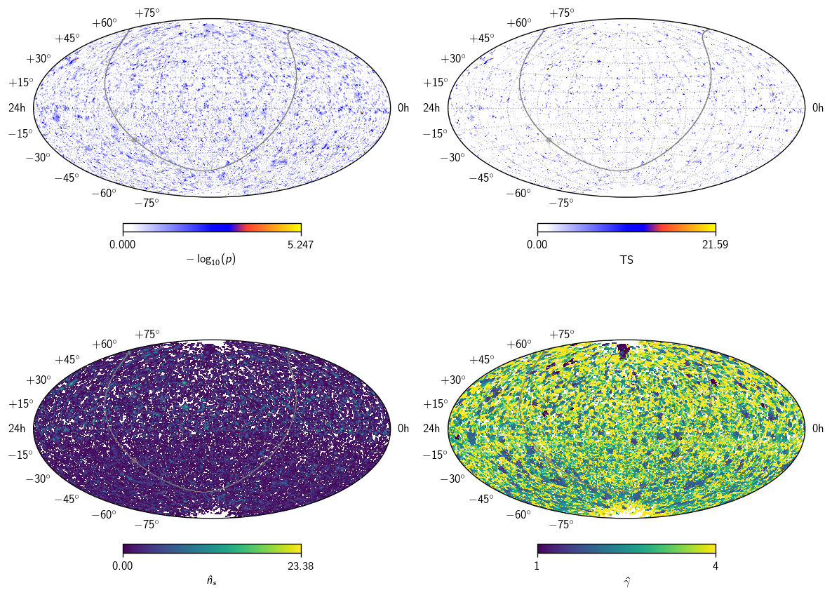
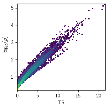
As you can see, the p-values are largely but not perfectly correlated with TS – as expected, since the background distributions vary with declination:

[39]:

fig, ax = plt.subplots(figsize=(3, 3))
hl.plot2d(ax, hl.hist((scan[1], scan[0]), bins=100), log=True)
ax.set_xlabel(r'TS')
ax.set_ylabel(r'$-\log_{10}(p)$')
plt.tight_layout()

All-sky scan: on the cluster 

This is pretty much the end of the road for this tutorial. Similar methods to those above can be used to run all-sky scans on the cluster. The analyzer needs to make her own determination regarding how much information to save and how. For example, SkyScanTrialRunner can simply return information about the hottest spot for each trial, much as an ordinary TrialRunner returns the best fit rather than a scan over a likelihood space:

[40]:

sstr_16 = cy.get_sky_scan_trial_runner(nside=16, min_dec=-rad85, max_dec=rad85, ts_to_p=ts_to_p)

[41]:

ss_trials = sstr_16.get_many_fits(10, mp_cpus=10)

Performing 10 background trials using 10 cores:
         10/10 trials complete.

[42]:

ss_trials.as_dataframe

[42]:

	dec	gamma	mlog10p	ns	ra	ts
0	-0.894583	2.275326	3.399392	8.279833	5.256126	12.130737
1	-0.572419	3.316402	3.472688	10.036256	2.847068	10.729564
2	-0.041679	3.145972	3.664444	14.406262	1.668971	13.456195
3	-1.054780	3.922119	4.188652	10.515437	5.262168	15.164125
4	-0.523599	4.000000	4.966873	13.138896	2.699806	17.995175
5	0.000000	3.433455	3.499141	17.676977	2.405282	13.733677
6	-0.622827	2.423386	3.530386	10.082906	6.135923	10.614528
7	0.840223	2.826246	3.134401	13.705542	3.534292	11.802156
8	-0.840223	2.624530	3.388785	12.279441	2.524494	12.484693
9	-0.083430	2.085589	3.940884	13.425646	0.539961	12.689423

However, you might want to see the maps for yourself to get a feel for whether they function as expected. You might need more than just hottest spot information if you plan to apply some sort of population analysis or a custom spatial prior method. And anyways, modern analyses use much more data, even better angular resolution, sometimes time-dependent likelihoods, all of which mean the required compute time is increased (in the case of improved resolution, the problem is that higher pixel density is required). So most likely, the question isn’t how many scans you can do per job, but how many jobs you will need for each scan.

csky doesn’t yet offer a dedicated, built-in scan-splitting approach, but this can be achieved by setting min_dec and max_dec values such that jobs with equal random seed are broken up into declination bands.

In any case, regardless of the specific approach chosen, the final step in a traditional all sky scan is to compute a post-trials p-value. This is done by finding the fraction of background-only skies with a hottest spot of greater than or equal to the hottest \(-\log_{10}(p)\) in the real unblinded map.

Before unblinding, sanity checks include but may not be limited to:

Is nside large enough? (values should vary smoothly from pixel to pixel)
Is the hottest-spot \(\sin(\delta)\) uniformly distributed?
Can the post-trials correction distribution be obtained in reasonable compute time?

Timing summary 

[43]:

print(timer)

ana setup                         | 0:00:02.993551
bg trials                         | 0:00:57.027624
signal trials                     | 0:07:15.878014
load bg trials                    | 0:00:02.611293
load sig trials                   | 0:00:00.832596
setup trial runners for sens/disc | 0:00:01.046077
compute sensitivity               | 0:00:01.763108
compute discovery potential       | 0:00:01.817958
unblind all-sky scan              | 0:02:37.720980
--------------------------------------------------
total                             | 0:11:01.691201

Remarks 

In this tutorial, we’ve offered some tips on how to scale up an analysis from interactive exploration to serious cluster computing. We’ve looked specifically at the use case of a time-integrated all-sky scan with declination-dependent background. However, the methods used here should be widely applicable for single-hypothesis analyses (stacking, template, special-case follow-ups, etc.) as well as for time-dependent analyses.

I (M. Richman) explicitly encourage users to discuss implementation details such as scripting command line interfaces, working with specific clusters, etc. on Slack under #csky! And by all means: if you come up with different, maybe even more elegant ways of dealing with trial data on disk, let us know — it’s possible that your methods would make a nice addition to cy.bk.