Spatial Priors

In this tutorial, we’ll give an overview of how to perform spatial prior analysis.

import numpy as np
import matplotlib.pyplot as plt
import healpy as hp

import histlite as hl
import csky as cy

%matplotlib inline

cy.plotting.mrichman_mpl()

ana_dir = '/data/user/mrichman/csky_cache/ana'

We’ll test with one year of data, PS IC86-2011.

ana = cy.get_analysis(cy.selections.repo, 'version-003-p02', cy.selections.PSDataSpecs.ps_2011, dir=ana_dir)

Setting up Analysis for:
IC86_2011
Setting up IC86_2011...
<- /data/user/mrichman/csky_cache/ana/IC86_2011.subanalysis.version-003-p02.npy
Done.

Everything that follows will use this same Analysis, so we put it in cy.CONF.

cy.CONF['ana'] = ana

Arbitrary prior

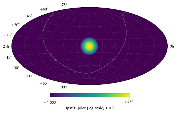
We’ll use histlite to create an arbitrary prior:

m = hl.heal.hist(128, [0], [np.pi]).smoothing(np.radians(10)).normalize()
m.map = np.maximum(1e-4, m.map)

fig, ax = plt.subplots (subplot_kw=dict (projection='aitoff'))
sp = cy.plotting.SkyPlotter(pc_kw=dict())
mesh, cb = sp.plot_map(ax, np.log10(m.map), n_ticks=2)
kw = dict(color='.5', alpha=.5)
sp.plot_gp(ax, lw=.5, **kw)
sp.plot_gc(ax, **kw)
ax.grid(**kw)
cb.set_label(r'spatial prior (log scale, a.u.)')
plt.tight_layout()

SpatialPriorTrialRunner

We’ll test using an nside=64 version of the prior map, just to keep things snappy.

We also need to give it a value for src_tr, to keep the spatial prior trial runner happy. Here, we’ll pass it ra=pi, dec=0.0, which is the best-fit of the map we made. We also need to keep the energy in the conf, for running trials.

prior = np.where(m.map >= m.map.min(), m.map, 0)
dec85 = np.radians(85)
sptr = cy.get_spatial_prior_trial_runner(llh_priors=hp.ud_grade(m.map, 64), min_dec=-dec85, max_dec=dec85,
                                         src_tr=cy.sources(np.pi,0.), conf={"extra_keep":["energy"]})

Now we can run a trial straight away:

%time result = sptr.get_one_fit(20, seed=1, mp_cpus=15, logging=True)
result

Scanning 48984 locations using 15 cores:
      48984/48984 coordinates complete.
CPU times: user 598 ms, sys: 376 ms, total: 974 ms
Wall time: 1min 1s

array([4.70029474e+01, 4.70029474e+01, 2.30528063e+01, 2.21504501e+00,
       2.96978681e+00, 1.04168551e-02])

Here we’ve got mlog10p,ts,ns,gamma,ra_best,dec_best:

print('TS, ns, gamma (ra,dec) = {:.2f}, {:.2f}, {:.2f} ({:.2f}, {:.2f})'.format(
    result[1], result[2], result[3], *np.degrees(result[-2:])))

TS, ns, gamma (ra,dec) = 47.00, 23.05, 2.22 (170.16, 0.60)

All-sky scans are slow

SpatialPriorTrialRunner allows the usual get_many_fits(), etc., but in practice this is almost useless if the trials are very slow such that they require one or more cluster jobs to complete in reasonable time. Therefore, it’s more likely that you’ll want to get the trial using SpatialPriorTrialRunner and run the scans using SkyScanTrialRunner.

To get the trial, we can say:

trial = sptr.get_one_trial(20, seed=1)
trial

SpatialPriorTrial(evss=[[Events(136244 items | columns: dec, energy, idx, inj, log10energy, ra, sigma, sindec), Events(20 items | columns: dec, energy, idx, inj, log10energy, ra, sigma, sindec)]], n_exs=[0], ra=array([2.96978681]), dec=array([0.01041686]))

Note that this also allows us to inspect the true source position(s) selected for this trial:

np.degrees([trial.ra, trial.dec]).ravel()

array([170.15625   ,   0.59684183])

In the above scan, the implicit trial was the same as this one, since the random seed was the same. And sure enough, the hottest point in the sky, after accounting for the prior, was at the position of the source.

We can reproduce that result by performing the all-sky scan manually:

sstr = cy.get_sky_scan_trial_runner(nside=64, min_dec=-dec85, max_dec=dec85)

%time scan = sstr.get_one_scan_from_trial(trial, mp_cpus=15, logging=True)

Scanning 48984 locations using 15 cores:
      48984/48984 coordinates complete.
CPU times: user 275 ms, sys: 325 ms, total: 600 ms
Wall time: 58.7 s

scan.shape

(4, 49152)

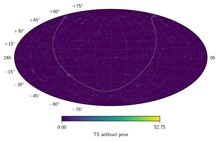
The 0th axis of this array has the elements mlog10p,ts,ns,gamma. The TS map looks like so:

fig, ax = plt.subplots (subplot_kw=dict (projection='aitoff'))
sp = cy.plotting.SkyPlotter(pc_kw=dict())
mesh, cb = sp.plot_map(ax, scan[1], n_ticks=2)
kw = dict(color='.5', alpha=.5)
sp.plot_gp(ax, lw=.5, **kw)
sp.plot_gc(ax, **kw)
ax.grid(**kw)
cb.set_label(r'TS without prior')
plt.tight_layout()

The TS map including the prior looks like so:

fig, ax = plt.subplots (subplot_kw=dict (projection='aitoff'))
sp = cy.plotting.SkyPlotter(pc_kw=dict())
ts_with_prior = scan[1] + sptr.llh_prior_term[0]
mesh, cb = sp.plot_map(ax, ts_with_prior, n_ticks=2)
kw = dict(color='.5', alpha=.5)
sp.plot_gp(ax, lw=.5, **kw)
sp.plot_gc(ax, **kw)
ax.grid(**kw)
cb.set_label(r'TS including prior')
plt.tight_layout()

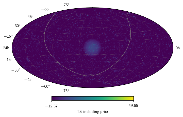
Notice that sptr.llh_prior_term[0] is for the 0th prior. If we had given multiple priors, they would have higher indices in this sequence.

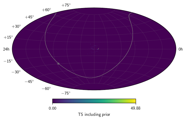
Now, if we disallow TS values below 0, we get:

fig, ax = plt.subplots (subplot_kw=dict (projection='aitoff'))
sp = cy.plotting.SkyPlotter(pc_kw=dict())
mesh, cb = sp.plot_map(ax, np.maximum(0, ts_with_prior), n_ticks=2)
kw = dict(color='.5', alpha=.5)
sp.plot_gp(ax, lw=.5, **kw)
sp.plot_gc(ax, **kw)
ax.grid(**kw)
cb.set_label(r'TS including prior')
plt.tight_layout()

Counts vs Flux

SpatialPriorTrialRunner supports counts \(\leftrightarrow\) flux conversions in much the same way as other trial runners. However, signal-injector-based conversions are not possible because the signal appears in a different position for each trial. So for example, the following is not possible:

sptr.to_E2dNdE(20, E0=100, unit=1e3)  # TeV/cm2/s @ 100TeV ?

---------------------------------------------------------------------------
AttributeError                            Traceback (most recent call last)
/tmp/ipykernel_29431/582389252.py in <module>
----> 1 sptr.to_E2dNdE(20, E0=100, unit=1e3)  # TeV/cm2/s @ 100TeV ?

/data/user/jthwaites/csky/csky/trial.py in to_E2dNdE(self, ns, flux, *a, **kw)
    212             * clarify sig_inj_acc_total vs get_acc_total situation in both code and docs
    213         """
--> 214         flux, params, fluxargs, acc = self._split_params_fluxargs_acc(flux, *a, **kw)
    215         return flux.to_E2dNdE(ns, acc, **fluxargs)
    216

/data/user/jthwaites/csky/csky/trial.py in _split_params_fluxargs_acc(self, flux, *a, **kw)
    157             flux = hyp.PowerLawFlux(params['gamma'])
    158         else:
--> 159             fluxs = np.atleast_1d(self.sig_injs[-1].flux)
    160             if not np.all(fluxs == fluxs[0]):
    161                 raise ValueError('cannot convert to mixed fluxes')

AttributeError: 'SpatialPriorTrialRunner' object has no attribute 'sig_injs'

But this is fine:

sptr.to_E2dNdE(20, E0=100, unit=1e3, gamma=2)  # TeV/cm2/s @ 100TeV !

1.0685320290882531e-11

This refers to the flux that would, on average, yield 20 events. Depending on the true source position, the flux might yield more or fewer events; but averaging over the spatial prior, this flux yields 20 events.

Remarks

Spatial prior analysis seems complex, but ultimately it just comes down to performing all-sky scans and penalizing the TS according to the prior.

Future work will include making it easy to restrict the pixel set that is evaluated and documenting how to do so. This is important for optimizing transient analyses where very few events are likely to be present, and only small time ranges need to be studied for ecah source.