Time-integrated stacking

In this tutorial we demonstrate time-integrated stacking analysis.

Setup 

[1]:

import numpy as np
import matplotlib.pyplot as plt
from scipy import stats

import histlite as hl
import csky as cy

%matplotlib inline

[2]:

cy.plotting.mrichman_mpl()

/mnt/lfs7/user/ssclafani/software/external/csky/csky/plotting.py:92: MatplotlibDeprecationWarning: Support for setting the 'text.latex.preamble' or 'pgf.preamble' rcParam to a list of strings is deprecated since 3.3 and will be removed two minor releases later; set it to a single string instead.
  r'\SetSymbolFont{operators}   {sans}{OT1}{cmss} {m}{n}'

Ideally we’d like to work with something like (Tessa’s) 10yr PS sample:

[3]:

ana_dir = cy.utils.ensure_dir('/data/user/mrichman/csky_cache/ana/')

[4]:

ana = cy.get_analysis(cy.selections.repo, 'version-003-p02', cy.selections.PSDataSpecs.ps_10yr, dir=ana_dir)

Setting up Analysis for:
IC40, IC59, IC79, IC86_2011, IC86v3_2012_2017
Setting up IC40...
Reading /data/ana/analyses/ps_tracks/version-003-p02/IC40_MC.npy ...
Reading /data/ana/analyses/ps_tracks/version-003-p02/IC40_exp.npy ...
Reading /data/ana/analyses/ps_tracks/version-003-p02/GRL/IC40_exp.npy ...
Energy PDF Ratio Model...
  * gamma = 4.0000 ...
Signal Acceptance Model...
  * gamma = 4.0000 ...
Setting up IC59...
Reading /data/ana/analyses/ps_tracks/version-003-p02/IC59_MC.npy ...
Reading /data/ana/analyses/ps_tracks/version-003-p02/IC59_exp.npy ...
Reading /data/ana/analyses/ps_tracks/version-003-p02/GRL/IC59_exp.npy ...
Energy PDF Ratio Model...
  * gamma = 4.0000 ...
Signal Acceptance Model...
  * gamma = 4.0000 ...
Setting up IC79...
Reading /data/ana/analyses/ps_tracks/version-003-p02/IC79_MC.npy ...
Reading /data/ana/analyses/ps_tracks/version-003-p02/IC79_exp.npy ...
Reading /data/ana/analyses/ps_tracks/version-003-p02/GRL/IC79_exp.npy ...
Energy PDF Ratio Model...
  * gamma = 4.0000 ...
Signal Acceptance Model...
  * gamma = 4.0000 ...
Setting up IC86_2011...
Reading /data/ana/analyses/ps_tracks/version-003-p02/IC86_2011_MC.npy ...
Reading /data/ana/analyses/ps_tracks/version-003-p02/IC86_2011_exp.npy ...
Reading /data/ana/analyses/ps_tracks/version-003-p02/GRL/IC86_2011_exp.npy ...
<- /data/user/mrichman/csky_cache/ana//IC86_2011.subanalysis.version-003-p02.npy
Setting up IC86v3_2012_2017...
Reading /data/ana/analyses/ps_tracks/version-003-p02/IC86_2012_MC.npy ...
Reading /data/ana/analyses/ps_tracks/version-003-p02/IC86_2012_exp.npy ...
Reading /data/ana/analyses/ps_tracks/version-003-p02/IC86_2013_exp.npy ...
Reading /data/ana/analyses/ps_tracks/version-003-p02/IC86_2014_exp.npy ...
Reading /data/ana/analyses/ps_tracks/version-003-p02/IC86_2015_exp.npy ...
Reading /data/ana/analyses/ps_tracks/version-003-p02/IC86_2016_exp.npy ...
Reading /data/ana/analyses/ps_tracks/version-003-p02/IC86_2017_exp.npy ...
Reading /data/ana/analyses/ps_tracks/version-003-p02/GRL/IC86_2012_exp.npy ...
Reading /data/ana/analyses/ps_tracks/version-003-p02/GRL/IC86_2013_exp.npy ...
Reading /data/ana/analyses/ps_tracks/version-003-p02/GRL/IC86_2014_exp.npy ...
Reading /data/ana/analyses/ps_tracks/version-003-p02/GRL/IC86_2015_exp.npy ...
Reading /data/ana/analyses/ps_tracks/version-003-p02/GRL/IC86_2016_exp.npy ...
Reading /data/ana/analyses/ps_tracks/version-003-p02/GRL/IC86_2017_exp.npy ...
<- /data/user/mrichman/csky_cache/ana//IC86v3_2012_2017.subanalysis.version-003-p02.npy
Done.

Taken together, this is just a lot of data.

[5]:

n_evs = np.array([len(a.data) for a in ana.anas])
n_ev = np.sum(n_evs)
n_ev, n_evs

[5]:

(1134451, array([ 36900, 107011,  93133, 136244, 761163]))

So instead we’ll do our test calculations with just the 2011 dataset, which is a little over 10% of the total 10yr ensemble:

[6]:

ana11 = cy.get_analysis(cy.selections.repo, cy.selections.PSDataSpecs.ps_2011, dir=ana_dir)

Setting up Analysis for:
IC86_2011
Setting up IC86_2011...
<- /data/user/mrichman/csky_cache/ana//IC86_2011.subanalysis.npy
Done.

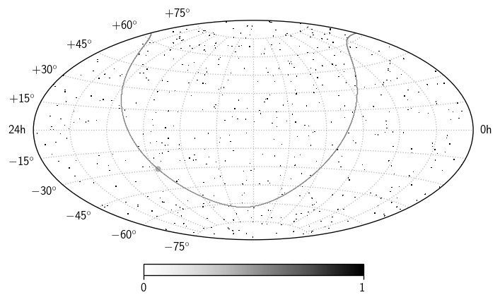
Of course, we’ll also need a catalog. Let’s just make one up, with 1k sources:

[7]:

N = 1000
np.random.seed(0)
src = cy.utils.Sources(
    ra=np.random.uniform(0, 2*np.pi, N),
    dec=np.arcsin(np.random.uniform(-1, 1, N)))

You can optionally include additional arrays of per-source extension (circular Gaussian, in radians) and weight.

We’ll quickly double check that the catalog is in fact random:

[12]:

src_map = hl.heal.hist(512, src.dec, src.ra)

[14]:

fig, ax = plt.subplots (subplot_kw=dict (projection='aitoff'))
sp = cy.plotting.SkyPlotter(pc_kw=dict(cmap='Greys', vmin=0))
mesh, cb = sp.plot_map(ax, np.where(src_map.map>0, src_map.map, np.nan), n_ticks=2)
kw = dict(color='.5', alpha=.5)
sp.plot_gp(ax, lw=.5, **kw)
sp.plot_gc(ax, **kw)
ax.grid(**kw)
plt.tight_layout()

_images/03_time_integrated_stacking_16_0.png

This setup should be basically all you need. We’ll leave it as an exercise for the reader to show that the compute time per trial scales approximately linearly with both \(N_\text{events}\) and \(N_\text{sources}\).

Background trials 

We start by constructing a trial runner. Note that we’re restricting the bandwidth from which signal events are drawn; this may be a premature optimization, but in principle this cuts down on RAM usage and CPU time taken by the signal injector.

[15]:

timer = cy.timing.Timer()
time = timer.time

[16]:

with time('trial runner construction'):
    tr = cy.get_trial_runner(src=src, ana=ana11, sindec_bandwidth=np.radians(.1), mp_cpus=20)

IC86_2011                                100%.

Let’s start with 200 trials:

[17]:

with time('bg trials (200)'):
    bg = cy.dists.Chi2TSD(tr.get_many_fits(200, seed=1))

Performing 200 background trials using 20 cores:
        200/200 trials complete.

Ok, this timing is manageable, so we flesh out the distribution a little more:

[18]:

with time('bg trials (+800)'):
    bg += cy.dists.Chi2TSD(tr.get_many_fits(800, seed=2))

Performing 800 background trials using 20 cores:
        800/800 trials complete.

We check the summary properties:

[19]:

print(bg)
print(bg.description)

Chi2TSD(1000 trials, eta=0.534, ndof=1.118, median=0.012 (from fit 0.010))
Chi2TSD from 1000 trials:
           eta = 0.534
          ndof = 1.118
           loc = 0.000
         scale = 0.847
Thresholds from trials:
        median = 0.012
       1 sigma = 1.06
       2 sigma = 3.73
       3 sigma = 8.05
       4 sigma = 14.04
       5 sigma = 21.71
Thresholds from fit:
        median = 0.010
       1 sigma = 1.06
       2 sigma = 3.73
       3 sigma = 8.05
       4 sigma = 14.04
       5 sigma = 21.71

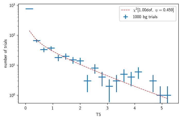
And then plot the distribution:

[82]:

fig, ax = plt.subplots()

h = bg.get_hist(bins=30)
hl.plot1d(ax, h, crosses=True, label='{} bg trials'.format(bg.n_total))

x = h.centers[0]
norm = h.integrate().values
ax.semilogy(x, norm * bg.pdf(x), lw=1, ls='--',
            label=r'$\chi^2[{:.2f}\text{{dof}},\ \eta={:.3f}]$'.format(bg.ndof, bg.eta))

ax.set_xlabel(r'TS')
ax.set_ylabel(r'number of trials')
ax.legend()
plt.tight_layout()

_images/03_time_integrated_stacking_29_0.png

Sensitivity 

First we confirm that the signal injector does anything at all:

[83]:

with time('single signal trial'):
    print(tr.get_one_fit(n_sig=100, seed=1))

CPU times: user 3.54 s, sys: 31.8 ms, total: 3.57 s
Wall time: 3.56 s

[83]:

[25.265407836196488, 168.1254497348161, 2.2607036848910664]

Seems legit. Now for sensitivity:

[20]:

with time('sensitivity'):
    sens = tr.find_n_sig(
        bg.median(), 0.9,
        n_sig_step=10,
        first_batch_size=20,
        batch_size=200,
        # 10% tolerance -- let's get an estimate quick!
        tol=.1,
        # number of signal signal strengths (default 6, i'm really tryina rush here)
        n_batches=5
    )

Start time: 2019-07-26 21:23:14.684362
Using 20 cores.
* Starting initial scan for 90% of 20 trials with TS >= 0.012...
  n_sig = 10.000 ... frac = 0.70000
  n_sig = 20.000 ... frac = 0.80000
  n_sig = 30.000 ... frac = 0.95000
* Generating batches of 200 trials...
n_trials | n_inj    0.00   15.00   30.00   45.00   60.00  |  n_sig(relative error)
200      |         45.0%   81.0%   95.5%   99.5%   99.5%  |     22.450 (+/-  5.4%) [spline]
End time: 2019-07-26 21:28:50.559238
Elapsed time: 0:05:35.874876

As a flux, this gives:

[21]:

tr.to_E2dNdE(sens, E0=100, unit=1e3)   # TeV/cm2/s  @  100TeV

[21]:

2.4410190834500614e-11

Timing summary 

[22]:

print(timer)

trial runner construction | 0:00:19.832247
bg trials (200)           | 0:00:58.479316
bg trials (+800)          | 0:03:33.984594
sensitivity               | 0:05:35.876342

Closing remarks 

Stacking is unavoidably computationally complex. In csky, we try to make it as fast as possible using the following optimizations:

The signal space PDF (including scrambled signal space PDF, if signal subtraction is desired) is computed in C++.
Only event-source pairs within \(n\,\sigma\) of each other (default: \(5\sigma\)) are computed in detail.
Included event-source pairs are managed using sparse matrices to dramatically reduce RAM usage. This is enabled automatically any time multiple sources are given.

Time-integrated stacking

Setup

Background trials

Sensitivity

Timing summary

Closing remarks

Setup 

Background trials 

Sensitivity 

Timing summary 

Closing remarks 