Implementation Inspection
In previous tutorials, we’ve taken a pragmatic approach to csky usage, demonstrating how to accomplish various analysis tasks. Here, we’ll look at how to access csky’s implementation details.
[2]:
import numpy as np
import matplotlib.pyplot as plt

import histlite as hl
import csky as cy

%matplotlib inline
[3]:
cy.plotting.mrichman_mpl()
/mnt/lfs7/user/ssclafani/software/external/csky/csky/plotting.py:92: MatplotlibDeprecationWarning: Support for setting the 'text.latex.preamble' or 'pgf.preamble' rcParam to a list of strings is deprecated since 3.3 and will be removed two minor releases later; set it to a single string instead.
  r'\SetSymbolFont{operators}   {sans}{OT1}{cmss} {m}{n}'
For these tests, let’s work with PS-7yr.
[ ]:
ana_dir = cy.utils.ensure_dir('/data/user/mrichman/csky_cache/ana')
ana = cy.get_analysis(cy.selections.repo, 'version-003-p02', cy.selections.PSDataSpecs.ps_7yr, dir=ana_dir)
Setting up Analysis for:
IC40, IC59, IC79, IC86_2011, IC86_2012_2014
Setting up IC40...
Reading /data/ana/analyses/ps_tracks/version-003-p02/IC40_MC.npy ...
Reading /data/ana/analyses/ps_tracks/version-003-p02/IC40_exp.npy ...
Reading /data/ana/analyses/ps_tracks/version-003-p02/GRL/IC40_exp.npy ...
Energy PDF Ratio Model...
  * gamma = 4.0000 ...
Signal Acceptance Model...
  * gamma = 4.0000 ...
Setting up IC59...
Reading /data/ana/analyses/ps_tracks/version-003-p02/IC59_MC.npy ...
Reading /data/ana/analyses/ps_tracks/version-003-p02/IC59_exp.npy ...
Reading /data/ana/analyses/ps_tracks/version-003-p02/GRL/IC59_exp.npy ...
Energy PDF Ratio Model...
  * gamma = 4.0000 ...
Signal Acceptance Model...
  * gamma = 4.0000 ...
Setting up IC79...
Reading /data/ana/analyses/ps_tracks/version-003-p02/IC79_MC.npy ...
Reading /data/ana/analyses/ps_tracks/version-003-p02/IC79_exp.npy ...
Reading /data/ana/analyses/ps_tracks/version-003-p02/GRL/IC79_exp.npy ...
Energy PDF Ratio Model...
  * gamma = 4.0000 ...
Signal Acceptance Model...
  * gamma = 1.0000 ...
Analysis Properties
In various situations, it may be useful to examine the Analysis itself. We can find out what “keys” are considered easily enough:
[4]:
ana
[4]:
Analysis(keys=[IC40, IC59, IC79, IC86_2011, IC86_2012_2014])
Each key corresponds to a SubAnalysis instance:
[5]:
for a in ana:
    print(a)
SubAnalysis(key=IC40)
SubAnalysis(key=IC59)
SubAnalysis(key=IC79)
SubAnalysis(key=IC86_2011)
SubAnalysis(key=IC86_2012_2014)
We can access individual SubAnalysiss directly:
[6]:
print(ana[0])
print(ana[-1])
print(ana['IC86_2012_2014'])
SubAnalysis(key=IC40)
SubAnalysis(key=IC86_2012_2014)
SubAnalysis(key=IC86_2012_2014)
And we can get a new Analysis with a subset of keys like so:
[7]:
ana[:-1] # same as ps_4yr
[7]:
Analysis(keys=[IC40, IC59, IC79, IC86_2011])
Each SubAnalysis holds references to the data, MC (signal Monte Carlo), GRL (Good Run List), background space PDF, energy PDF ratio model, and signal acceptance parameterization:
[8]:
a = ana[-1]
print(a.data)
print(a.sig)
print(a.grl)
print(a.bg_space_param)
print(a.energy_pdf_ratio_model)
print(a.acc_param)
Events(338590 items | columns: azimuth, dec, energy, event, log10energy, mjd, ra, run, sigma, sindec, subevent)
Events(6807254 items | columns: azimuth, dec, energy, event, log10energy, mjd, ra, run, sigma, sindec, subevent, xdec, xra, true_dec, true_energy, true_ra, oneweight)
Arrays(3931 items | columns: events, livetime, run, start, stop)
<csky.pdf.BgSinDecParameterization object at 0x7fd573043400>
<csky.pdf.EnergyPDFRatioModel object at 0x7fd573153860>
<csky.pdf.SinDecAccParameterization object at 0x7fd573095710>
We can look at the keyword arguments used to construct the latter three objects:
[9]:
print(a.kw_space_bg, '\n\n', a.kw_energy, '\n\n', a.kw_acc)
{'hkw': {'bins': array([-1.        , -0.9825    , -0.965     , -0.9475    , -0.93      ,
       -0.867     , -0.804     , -0.741     , -0.678     , -0.615     ,
       -0.552     , -0.489     , -0.426     , -0.363     , -0.3       ,
       -0.26111111, -0.22222222, -0.18333333, -0.14444444, -0.10555556,
       -0.06666667, -0.02777778,  0.01111111,  0.05      ,  0.10277778,
        0.15555556,  0.20833333,  0.26111111,  0.31388889,  0.36666667,
        0.41944444,  0.47222222,  0.525     ,  0.57777778,  0.63055556,
        0.68333333,  0.73611111,  0.78888889,  0.84166667,  0.89444444,
        0.94722222,  1.        ])}}

 {'hkw': {'bins': (array([-1.        , -0.9825    , -0.965     , -0.9475    , -0.93      ,
       -0.867     , -0.804     , -0.741     , -0.678     , -0.615     ,
       -0.552     , -0.489     , -0.426     , -0.363     , -0.3       ,
       -0.26111111, -0.22222222, -0.18333333, -0.14444444, -0.10555556,
       -0.06666667, -0.02777778,  0.01111111,  0.05      ,  0.10277778,
        0.15555556,  0.20833333,  0.26111111,  0.31388889,  0.36666667,
        0.41944444,  0.47222222,  0.525     ,  0.57777778,  0.63055556,
        0.68333333,  0.73611111,  0.78888889,  0.84166667,  0.89444444,
        0.94722222,  1.        ]), array([1.   , 1.125, 1.25 , 1.375, 1.5  , 1.625, 1.75 , 1.875, 2.   ,
       2.125, 2.25 , 2.375, 2.5  , 2.625, 2.75 , 2.875, 3.   , 3.125,
       3.25 , 3.375, 3.5  , 3.625, 3.75 , 3.875, 4.   , 4.125, 4.25 ,
       4.375, 4.5  , 4.625, 4.75 , 4.875, 5.   , 5.125, 5.25 , 5.375,
       5.5  , 5.625, 5.75 , 5.875, 6.   , 6.125, 6.25 , 6.375, 6.5  ,
       6.625, 6.75 , 6.875, 7.   , 7.125, 7.25 , 7.375, 7.5  , 7.625,
       7.75 , 7.875, 8.   , 8.125, 8.25 , 8.375, 8.5  , 8.625, 8.75 ,
       8.875, 9.   , 9.125, 9.25 , 9.375, 9.5  ]))}, 'gammas': array([1.    , 1.0625, 1.125 , 1.1875, 1.25  , 1.3125, 1.375 , 1.4375,
       1.5   , 1.5625, 1.625 , 1.6875, 1.75  , 1.8125, 1.875 , 1.9375,
       2.    , 2.0625, 2.125 , 2.1875, 2.25  , 2.3125, 2.375 , 2.4375,
       2.5   , 2.5625, 2.625 , 2.6875, 2.75  , 2.8125, 2.875 , 2.9375,
       3.    , 3.0625, 3.125 , 3.1875, 3.25  , 3.3125, 3.375 , 3.4375,
       3.5   , 3.5625, 3.625 , 3.6875, 3.75  , 3.8125, 3.875 , 3.9375,
       4.    ]), 'bg_from_mc_weight': ''}

 {'hkw': {'bins': array([-1.        , -0.9825    , -0.965     , -0.9475    , -0.93      ,
       -0.867     , -0.804     , -0.741     , -0.678     , -0.615     ,
       -0.552     , -0.489     , -0.426     , -0.363     , -0.3       ,
       -0.26111111, -0.22222222, -0.18333333, -0.14444444, -0.10555556,
       -0.06666667, -0.02777778,  0.01111111,  0.05      ,  0.10277778,
        0.15555556,  0.20833333,  0.26111111,  0.31388889,  0.36666667,
        0.41944444,  0.47222222,  0.525     ,  0.57777778,  0.63055556,
        0.68333333,  0.73611111,  0.78888889,  0.84166667,  0.89444444,
        0.94722222,  1.        ])}, 'gammas': array([1.    , 1.0625, 1.125 , 1.1875, 1.25  , 1.3125, 1.375 , 1.4375,
       1.5   , 1.5625, 1.625 , 1.6875, 1.75  , 1.8125, 1.875 , 1.9375,
       2.    , 2.0625, 2.125 , 2.1875, 2.25  , 2.3125, 2.375 , 2.4375,
       2.5   , 2.5625, 2.625 , 2.6875, 2.75  , 2.8125, 2.875 , 2.9375,
       3.    , 3.0625, 3.125 , 3.1875, 3.25  , 3.3125, 3.375 , 3.4375,
       3.5   , 3.5625, 3.625 , 3.6875, 3.75  , 3.8125, 3.875 , 3.9375,
       4.    ])}
There’s also some other metadata:
[10]:
print(a.key, a.plot_key, a.mjd_min, a.mjd_max, a.livetime)
IC86_2012_2014 IC86\_2012\_2014 56043.42668248483 57160.03913214595 91452557.81247967
Notice that a.plot_key is valid LaTeX for use in matplotlib labels. Also notice that livetime is given in seconds, which is appropriate for many weighting routines. This is inconsistent with the use of days for time PDFs, which is a little ugly, but tolerable, since time-dependent analyses rely on the GRL which holds livetime in days:
[11]:
a.grl.as_dataframe.head()
[11]:
| events | livetime | run | start | stop | |
|---|---|---|---|---|---|
| 0 | 108 | 0.333588 | 120028 | 56043.423125 | 56043.756713 |
| 1 | 103 | 0.333414 | 120029 | 56043.757211 | 56044.090625 |
| 2 | 100 | 0.333437 | 120030 | 56044.091296 | 56044.424734 |
| 3 | 93 | 0.280688 | 120156 | 56062.420712 | 56062.701400 |
| 4 | 91 | 0.333329 | 120157 | 56062.702321 | 56063.035649 |
By the way, this trick is useful for examining any Arrays, Events, or Sources instance: convert to a Pandas DataFrame, and exploit its cute tabular displays:
[12]:
# first few data events
a.data.as_dataframe.head()
[12]:
| azimuth | dec | energy | event | log10energy | mjd | ra | run | sigma | sindec | subevent | |
|---|---|---|---|---|---|---|---|---|---|---|---|
| 0 | 3.357385 | -0.993323 | 88445.054688 | 839634 | 4.946673 | 56043.426682 | 4.641696 | 120028 | 0.003491 | -0.837845 | 0 |
| 1 | 4.714813 | -0.139147 | 4839.037109 | 2957343 | 3.684759 | 56043.435620 | 3.340578 | 120028 | 0.006210 | -0.138698 | 0 |
| 2 | 0.069405 | 0.146224 | 636.111328 | 3122255 | 2.803533 | 56043.436319 | 1.707208 | 120028 | 0.016994 | 0.145703 | 0 |
| 3 | 5.216482 | -0.911558 | 110068.148438 | 3489657 | 5.041662 | 56043.437871 | 2.853088 | 120028 | 0.003491 | -0.790459 | 0 |
| 4 | 4.932652 | 0.403303 | 1070.047485 | 3578643 | 3.029403 | 56043.438247 | 3.139286 | 120028 | 0.009331 | 0.392459 | 2 |
[13]:
# highest energy sig MC events
sig = a.sig
sig[sig.log10energy > 9].as_dataframe
[13]:
| azimuth | dec | energy | event | log10energy | mjd | oneweight | ra | run | sigma | sindec | subevent | true_dec | true_energy | true_ra | xdec | xra | |
|---|---|---|---|---|---|---|---|---|---|---|---|---|---|---|---|---|---|
| 0 | 1.279314 | -0.228347 | 1.360283e+09 | 385 | 9.133630 | 55927.019676 | 3.574832e+11 | 2.159943 | 1107000161 | 0.085668 | -0.226368 | 0 | -0.227076 | 1.128383e+08 | 2.230105 | -0.001811 | -0.068338 |
| 1 | 5.496354 | -0.264553 | 1.694245e+09 | 142 | 9.228976 | 55927.019676 | 3.858964e+12 | 4.226089 | 1107000598 | 0.018461 | -0.261478 | 0 | -0.281237 | 7.236306e+08 | 4.468642 | 0.008842 | -0.233963 |
| 2 | 1.602643 | -0.958788 | 1.012432e+09 | 389 | 9.005366 | 55927.019676 | 2.402457e+12 | 1.836615 | 1107002307 | 0.018874 | -0.818496 | 0 | -0.985183 | 8.687488e+08 | 1.808550 | 0.026207 | 0.016128 |
| 3 | 4.980302 | -0.899275 | 1.076434e+09 | 33 | 9.031987 | 55927.019676 | 2.874464e+12 | 4.742141 | 1107002576 | 0.061426 | -0.782876 | 0 | -0.836727 | 9.506101e+08 | 4.833335 | -0.064472 | -0.056809 |
| 4 | 1.666342 | -0.281335 | 1.094350e+09 | 260 | 9.039156 | 55927.019676 | 4.426455e+12 | 1.772916 | 1107003398 | 0.038012 | -0.277638 | 0 | -0.234172 | 7.059776e+08 | 1.705232 | -0.047674 | 0.065093 |
| 5 | 5.639177 | -0.147922 | 1.403493e+09 | 133 | 9.147210 | 55927.019676 | 3.658860e+12 | 4.083266 | 1107003839 | 0.031450 | -0.147383 | 0 | -0.144847 | 4.670470e+08 | 4.120126 | -0.003172 | -0.036458 |
As a quick aside, you may be wondering why, then, do the Arrays etc. classes even exist? The main reason is full-speed computation without writing (whatever).values all over the place:
[14]:
# Arrays
n, N = 100000, len(a.data)
%timeit ignore = np.sin(a.data.dec[np.random.randint(N, size=n)])
2.37 ms ± 94.2 µs per loop (mean ± std. dev. of 7 runs, 100 loops each)
[15]:
# DataFrame
df_data = a.data.as_dataframe
%timeit ignore = np.sin(df_data.dec[np.random.randint(N, size=n)])
171 ms ± 17.3 ms per loop (mean ± std. dev. of 7 runs, 10 loops each)
[16]:
# DataFrame, accessing .values
df_data = a.data.as_dataframe
%timeit ignore = np.sin(df_data.dec.values[np.random.randint(N, size=n)])
2.39 ms ± 57.2 µs per loop (mean ± std. dev. of 7 runs, 100 loops each)
There may be ways to make DataFrames fast enough for our applications, but we’re already doing lots of custom array manipulation, so it’s easier to use something that doesn’t detour through Pandas’s concept of data Series.
Analysis summary table recipies
Here are some snippets for quickly getting summary info on your datasets:
[17]:
print('Livetimes:')
for a in ana:
    print('{:20} {:.6f} {:.6f} ({:.2f} days)'.format(
        a.key, a.mjd_min, a.mjd_max, a.livetime/86400))
Livetimes:
IC40                 54562.379113 54971.132791 (376.36 days)
IC59                 54971.158700 55347.275122 (353.58 days)
IC79                 55348.314439 55694.405063 (316.05 days)
IC86_2011            55694.991910 56062.416216 (332.96 days)
IC86_2012_2014       56043.426682 57160.039132 (1058.48 days)
[18]:
print('Event Statistics:')
for a in ana:
    print('{:20} {:6} events in {} runs ({} MC events)'.format(
        a.key, len(a.data), len(a.grl), len(a.sig)))
Event Statistics:
IC40                  36900 events in 1420 runs (621858 MC events)
IC59                 107011 events in 1238 runs (1617012 MC events)
IC79                  93133 events in 1049 runs (1998573 MC events)
IC86_2011            136244 events in 1081 runs (1242934 MC events)
IC86_2012_2014       338590 events in 3931 runs (6807254 MC events)
[19]:
print('Number of sindec and log10energy bins:')
for a in ana:
    eprm = a.energy_pdf_ratio_model
    print('{:20} {:2} x {:2}'.format(
        a.key, *eprm.h_bg.n_bins))
Number of sindec and log10energy bins:
IC40                 30 x 56
IC59                 52 x 60
IC79                 49 x 56
IC86_2011            28 x 72
IC86_2012_2014       41 x 68
csky could, in principle, include functions to produce these tables. However, it’s probably best to simply understand enough of (1) the SubAnalysis internals, and (2) str.format(), such that you can produce your own tables on an as-needed basis.
Per-trial details
First things first: let’s get a simple time-integrating trial runner:
[20]:
src = cy.sources(180, 0, deg=True)
[21]:
tr = cy.get_trial_runner(src=src, ana=ana)
We already saw in Getting started with csky that we can get the trial data:
[22]:
trial = tr.get_one_trial(n_sig=100, poisson=False, seed=1)
tuple(trial)
[22]:
([[Events(3635 items | columns: dec, idx, inj, log10energy, ra, sigma, sindec),
   Events(8 items | columns: dec, idx, inj, log10energy, ra, sigma, sindec)],
  [Events(10335 items | columns: dec, idx, inj, log10energy, ra, sigma, sindec),
   Events(15 items | columns: dec, idx, inj, log10energy, ra, sigma, sindec)],
  [Events(8976 items | columns: dec, idx, inj, log10energy, ra, sigma, sindec),
   Events(4 items | columns: dec, idx, inj, log10energy, ra, sigma, sindec)],
  [Events(12322 items | columns: dec, idx, inj, log10energy, ra, sigma, sindec),
   Events(18 items | columns: dec, idx, inj, log10energy, ra, sigma, sindec)],
  [Events(26507 items | columns: dec, idx, inj, log10energy, ra, sigma, sindec),
   Events(55 items | columns: dec, idx, inj, log10energy, ra, sigma, sindec)]],
 [33265, 96676, 84157, 123922, 312083])
And that we can construct a likelihood evaluator (for multi-dataset analysis, a MultiLLHEvaluator) either directly or from this trial:
[23]:
L = tr.get_one_llh(n_sig=100, poisson=False, seed=1)
L.fit(**tr.fitter_args)
[23]:
(309.90800833895474, {'gamma': 2.0897522380963123, 'ns': 105.15666984028661})
[24]:
L = tr.get_one_llh_from_trial(trial)
L.fit(**tr.fitter_args)
[24]:
(309.90800833895474, {'gamma': 2.0897522380963123, 'ns': 105.15666984028661})
Between trial and L, we have access to all the likelihood implementation details. We discuss these in turn, below.
Trial data
Let’s talk a little more about the trial here. This is an instance of Trial, which is a “named tuple” (see collections.namedtuple). Within csky, it can be used interchangeably with a standard 2-tuple (that is, a tuple with 2 elements).
The first element is a sequence with one list per dataset. Each list includes at least the background events and possibly also some signal events:
[25]:
for evs in trial.evss:
    for ev in evs:
        print(ev)
    print()
Events(3635 items | columns: dec, idx, inj, log10energy, ra, sigma, sindec)
Events(8 items | columns: dec, idx, inj, log10energy, ra, sigma, sindec)

Events(10335 items | columns: dec, idx, inj, log10energy, ra, sigma, sindec)
Events(15 items | columns: dec, idx, inj, log10energy, ra, sigma, sindec)

Events(8976 items | columns: dec, idx, inj, log10energy, ra, sigma, sindec)
Events(4 items | columns: dec, idx, inj, log10energy, ra, sigma, sindec)

Events(12322 items | columns: dec, idx, inj, log10energy, ra, sigma, sindec)
Events(18 items | columns: dec, idx, inj, log10energy, ra, sigma, sindec)

Events(26507 items | columns: dec, idx, inj, log10energy, ra, sigma, sindec)
Events(55 items | columns: dec, idx, inj, log10energy, ra, sigma, sindec)
[26]:
trial.evss is trial[0]
[26]:
True
Notice that the signal events are split among the datasets probabilistically in accordance with the relative signal acceptance of each dataset. For reference, those relative weights are:
[27]:
print(tr.sig_inj_probs)
[0.08246462 0.13296804 0.15242021 0.17622968 0.45591745]
which are just a sum-to-one normalized version of the total signal acceptances:
[28]:
print(tr.sig_inj_accs)
print(tr.sig_inj_accs / tr.sig_inj_acc_total)
[9.97411814e+08 1.60825199e+09 1.84352646e+09 2.13150271e+09
 5.51433365e+09]
[0.08246462 0.13296804 0.15242021 0.17622968 0.45591745]
Anyways, we see that the background Events are only a small subset of the total datasets:
[29]:
for (j, a) in enumerate(ana):
    print('{:20} evaluating on {:5} of {:6} events'.format(
        a.key, len(trial[0][j][0]), len(a.data)))
IC40                 evaluating on  3635 of  36900 events
IC59                 evaluating on 10335 of 107011 events
IC79                 evaluating on  8976 of  93133 events
IC86_2011            evaluating on 12322 of 136244 events
IC86_2012_2014       evaluating on 26507 of 338590 events
The discrepancy is thanks to csky’s aggressively optimized “band” cuts, where events more than 5σ away from the source in declination are not included — cutting based on per-event angular error σ. The LLHEvaluators need to know how many events were excluded by these cuts, and this info is stored in trial.n_exs (as in, plural of “n excluded”; same as trial[1]):
[30]:
print(trial.n_exs)
print(trial[1])
[33265, 96676, 84157, 123922, 312083]
[33265, 96676, 84157, 123922, 312083]
Let’s confirm that these numbers agree with the missing events listed above:
[31]:
for (j, a) in enumerate(ana):
    Nj, nj = len(a.data), len(trial[0][j][0])
    print('{:20} {:6} - {:5} = {:6} | compare with {:6}'.format(
        a.key, Nj, nj, Nj - nj, trial[1][j]))
IC40                  36900 -  3635 =  33265 | compare with  33265
IC59                 107011 - 10335 =  96676 | compare with  96676
IC79                  93133 -  8976 =  84157 | compare with  84157
IC86_2011            136244 - 12322 = 123922 | compare with 123922
IC86_2012_2014       338590 - 26507 = 312083 | compare with 312083
For now, just take my word for it that even though these are calculable in this case, it’s important that trial.n_exs keeps track of these numbers.
From the Events objects, we can actually trace the origin of each individual event:
[32]:
print(trial.evss[0][0])
print(trial.evss[0][0].inj[0])
Events(3635 items | columns: dec, idx, inj, log10energy, ra, sigma, sindec)
<csky.inj.DataInjector object at 0x7fd57306d6d8>
Here, for example, we find that… well, the IC40 DataInjector had been used. To confirm:
[33]:
print(tr.bg_injs[0])
print(tr.bg_injs[0] is trial.evss[0][0].inj[0])
<csky.inj.DataInjector object at 0x7fd57306d6d8>
True
Of course, we can check this for all background and signal events:
[34]:
for (i, a) in enumerate(ana):
    print('{:20}  bg matches? {}'.format(a.key, tr.bg_injs[i] is trial.evss[i][0].inj[0]))
    print('{:20} sig matches? {}'.format(a.key, tr.sig_injs[i] is trial.evss[i][1].inj[0]))
IC40                  bg matches? True
IC40                 sig matches? True
IC59                  bg matches? True
IC59                 sig matches? True
IC79                  bg matches? True
IC79                 sig matches? True
IC86_2011             bg matches? True
IC86_2011            sig matches? True
IC86_2012_2014        bg matches? True
IC86_2012_2014       sig matches? True
We can quickly sanity check our signal events. For example, are they all in the right place spatially?
[35]:
all_sig_ev = cy.utils.Arrays.concatenate([evs[1] for evs in trial.evss])
hl.plot2d(hl.kde((all_sig_ev.ra_deg, all_sig_ev.dec_deg), range=((178, 182), (-2, 2))))
plt.gca().set_aspect('equal')
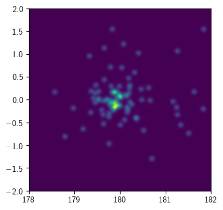
Note that if the above syntax doesn’t work, your histlite is probably out of date. Install the latest from PyPI – in your terminal,
pip uninstall histlite
pip install --user histlite
Alright, let’s move on to the actual likelihood.
PDFs and Likelihood
The likelihood is expressed as a MultiLLHEvaluator,
[36]:
L
[36]:
<csky.llh.MultiLLHEvaluator at 0x7fd572ffa9b0>
which is essentially a sequence of LLHEvaluator, plus some extra plumbing for multi-dataset analysis:
[37]:
for l in L:
    print(l)
<csky.llh.LLHEvaluator object at 0x7fd572ffa748>
<csky.llh.LLHEvaluator object at 0x7fd5730379b0>
<csky.llh.LLHEvaluator object at 0x7fd573037e10>
<csky.llh.LLHEvaluator object at 0x7fd573037cf8>
<csky.llh.LLHEvaluator object at 0x7fd572ff8080>
From either a TrialRunner or a MultiLLHEvaluator, we can access the LLH model, PDF ratio models (parameterizations, etc.), and evaluators (number crunchers) using cy.inspect. Here are some PDF ratio model examples, using index -1, corresponding to the 2012-2014 dataset:
[38]:
print('From the TrialRunner:')
print(cy.inspect.get_llh_model(tr, -1))
print(cy.inspect.get_pdf_ratio_model(tr, -1))
print(cy.inspect.get_space_model(tr, -1))
print(cy.inspect.get_energy_model(tr, -1))
From the TrialRunner:
<csky.llh.LLHModel object at 0x7fd572ffafd0>
<csky.pdf.MultiPDFRatioModel object at 0x7fd572ffaf60>
<csky.pdf.PointSourceSpacePDFRatioModel object at 0x7fd572ffa278>
<csky.pdf.EnergyPDFRatioModel object at 0x7fd573153860>
[39]:
print('From the MultiLLHEvaluator:')
print(cy.inspect.get_llh_model(L, -1))
print(cy.inspect.get_pdf_ratio_model(L, -1))
print(cy.inspect.get_space_model(L, -1))
print(cy.inspect.get_energy_model(L, -1))
From the MultiLLHEvaluator:
<csky.llh.LLHModel object at 0x7fd572ffafd0>
<csky.pdf.MultiPDFRatioModel object at 0x7fd572ffaf60>
<csky.pdf.PointSourceSpacePDFRatioModel object at 0x7fd572ffa278>
<csky.pdf.EnergyPDFRatioModel object at 0x7fd573153860>
Since this is a time-integrating setup, we won’t be able to find a time PDF ratio model:
[40]:
# would work if we were doing time-dep analysis!
cy.inspect.get_time_model(L, -1)
---------------------------------------------------------------------------
TypeError                                 Traceback (most recent call last)
<ipython-input-40-33329eeff7d6> in <module>()
      1 # would work if we were doing time-dep analysis!
----> 2 cy.inspect.get_time_model(L, -1)

/mnt/lfs3/user/mrichman/software/python/csky/csky/inspect.py in get_time_model(L, key)
     54         return acc_model.time_model
     55     else:
---> 56         raise TypeError('time model not found')
     57
     58 def get_energy_model(L, key=0):

TypeError: time model not found
Now, we can also get the PDF ratio evaluators, and this is where the interesting work happens:
[41]:
space_eval = cy.inspect.get_space_eval(L, -1, 0) # 0: background events (1 would be for signal events)
energy_eval = cy.inspect.get_energy_eval(L, -1, 0)
print(space_eval)
print(energy_eval)
<csky.pdf.PointSourceSpacePDFRatioEvaluator object at 0x7fd572ff85f8>
<csky.pdf.EnergyPDFRatioEvaluator object at 0x7fd572ff86d8>
Again, we won’t be able to get a time evaluator:
[42]:
# would work if we were doing time-dep analysis!
cy.inspect.get_time_eval(L, -1, 0)
---------------------------------------------------------------------------
TypeError                                 Traceback (most recent call last)
<ipython-input-42-15469da2593a> in <module>()
      1 # would work if we were doing time-dep analysis!
----> 2 cy.inspect.get_time_eval(L, -1, 0)

/mnt/lfs3/user/mrichman/software/python/csky/csky/inspect.py in get_time_eval(L, key, i)
     89         return eval
     90     else:
---> 91         raise TypeError('time evaluator not found')
     92
     93 def get_energy_eval(L, key=0, i=0):

TypeError: time evaluator not found
From here, we can access the actual PDF values that go into the likelihood. These evaluators act as functions when called. The allowed argments are parameters that go into the fit, and they are accepted only as keyword arguments. Each evaluator only strictly requires parameters it cares about — meanwhile, they all ignore parameters that they do not depend on. When called, two arrays are returned: the ordinary \(S/B\), and the signal subtraction \(\tilde{S}/B\), where \(\tilde{S}\) is the right-ascension-averaged signal PDF. Note that \(S\) and \(\tilde{S}\) differ only for space.
[43]:
print(space_eval()[0][:4])
print(space_eval()[1][:4])
print(energy_eval(gamma=2)[0][:4])
print(energy_eval(gamma=2)[1][:4])
[1.88494265e+00 4.63178921e+00 6.74842346e+02 5.78967374e-05]
[1.53234816 0.25578275 9.74167442 0.71069479]
[ 0.61933755  0.61088566  4.10332275 82.95478122]
[ 0.61933755  0.61088566  4.10332275 82.95478122]
So, for example, we can plot the space and energy PDF ratio distributions, where we’ll consider \(E^{-2}\) for the latter:
[44]:
SB_space = space_eval()[0]
SB_energy = energy_eval(gamma=2)[0]
[45]:
fig, axs = plt.subplots(1, 2, figsize=(7,3))
hl.plot1d(axs[0], hl.hist(SB_space, bins=50, log=True), crosses=True)
hl.plot1d(axs[1], hl.hist(SB_energy, bins=50, log=True), crosses=True)
for ax in axs:
    ax.loglog()
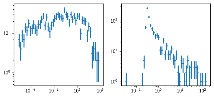
We should check how many values we got:
[46]:
SB_space.size, SB_energy.size, len(trial.evss[-1][0]), len(ana[-1].data)
[46]:
(879, 879, 26507, 338590)
Ok — it’s natural that the PDF ratio arrays are aligned with each other. But why so many fewer events than in the already-cut trial data? This is because csky applies a “box” cut that is equally aggressive as the earlier “band” cut, but this time in terms of distance to the source in right ascension.
If we want to evaluate on specific Events (maybe imported from skylab or hand-constructed for some test) we can instead work with fresh evaluators constructed on the fly. Notice that here the “band” cut is already reflected in the Events object, but the “box” cut is not applied:
[47]:
# 2012-2014 background events
ev = trial.evss[-1][0]
space_model = cy.inspect.get_space_model(tr)
# space_model(ev) -> PointSourceSpacePDFRatioEvaluator
print(space_model(ev)()[0].size)
26507
The “box” cut is computed by PointSourceSpacePDFRatioEvaluator, but is not applied before results are requested. Application of cuts is managed by MultiPDFRatioEvaluator in a way that preserves array alignment across the space, energy, and time PDFs. Internally, that looks something like this:
[48]:
# get the evaluator for 2012-2014 background events
se = space_model(ev)
# finalize the event list
kept_i_ev = se.get_kept_i_ev()
se.finalize_i_ev(kept_i_ev)
# now we see the box cut has been applied
se()[0].size
[48]:
879
For detailed low-level studies, it can be useful to evaluate the PDFs on every single event, especially if comparing with another tool (e.g. skylab, skyllh) where array alignment will be difficult after applying cuts. For this, however, we need a slightly different trial runner configuration:
[49]:
tr_uncut = cy.get_trial_runner(src=src, ana=ana, cut_n_sigma=np.inf)
This trial runner will, of course, be much slower to use, but now it will be possible to examine the response to every event. Here, we’ll include signal events on the plot:
[50]:
L_uncut = tr_uncut.get_one_llh(n_sig=1000, poisson=False, seed=1)
[51]:
fig, axs = plt.subplots(1, 2, figsize=(7,3))

for bg_or_sig in (0, 1):
    space_eval_uncut = cy.inspect.get_space_eval(L_uncut, -1, bg_or_sig)
    energy_eval_uncut = cy.inspect.get_energy_eval(L_uncut, -1, bg_or_sig)
    SB_space_uncut = space_eval_uncut()[0]
    SB_energy_uncut = energy_eval_uncut(gamma=2)[0]
    kw = dict(bins=50, range=(1e-10, 1e10), log=True)
    hl.plot1d(axs[0], hl.hist(SB_space_uncut, **kw), crosses=True)
    hl.plot1d(axs[1], hl.hist(SB_energy_uncut, **kw), crosses=True)
for ax in axs:
    ax.loglog()
    ax.axvline(1, color='k', ls='--', lw=1, zorder=-10)
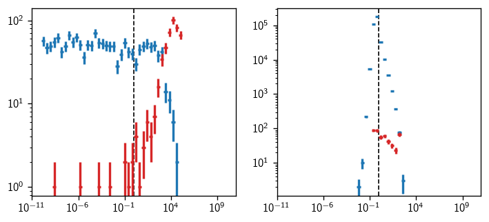
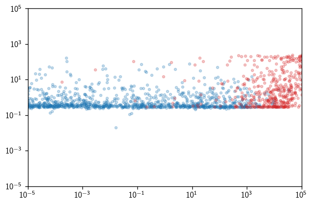
If you have skylab up and running simultaneously, and you know how to extract its PDF ratios, then you can make useful scatterplots comparing arrays like SB_space_uncut and SB_energy_uncut with the skylab equivalents. We aren’t doing that in this tutorial, so here’s a sillier plot comparing the space and energy PDF ratios:
[52]:
fig, ax = plt.subplots()

for bg_or_sig in (0, 1):
    space_eval_uncut = cy.inspect.get_space_eval(L_uncut, -1, bg_or_sig)
    energy_eval_uncut = cy.inspect.get_energy_eval(L_uncut, -1, bg_or_sig)
    SB_space_uncut = space_eval_uncut()[0]
    SB_energy_uncut = energy_eval_uncut(gamma=2)[0]
    ax.loglog(SB_space_uncut, SB_energy_uncut, '.', alpha=.25)
ax.set_xlim(1e-5, 1e5)
ax.set_ylim(1e-5, 1e5)
[52]:
(1e-05, 100000.0)
Likelihood confirmation
It turns out that it’s actually pretty easy to confirm the underlying likelihood implementation by writing it from scratch. Let’s get the fit for 2012-2014 only:
[53]:
L_uncut[-1].fit(**tr_uncut.fitter_args)
[53]:
(2933.922943418569, {'gamma': 1.999080216432319, 'ns': 445.0750138559467})
(Oh, right, we injected lots of signal into this trial.) Ok, now let’s get the space and energy PDFs (for the best-fit spectrum) as well as the overall \(S/B\):
[54]:
# concatenate background and signal S/B values
SB_space = np.concatenate([cy.inspect.get_space_eval(L_uncut, -1, i)()[0] for i in (0, 1)])
SB_energy = np.concatenate([cy.inspect.get_energy_eval(L_uncut, -1, i)(gamma=1.999)[0] for i in (0, 1)])
SB = SB_space * SB_energy
Now we can write down the test statistic as a function of ns:
[55]:
# np.vectorize in case we wanted to call for an array of ns
@np.vectorize
def ts(ns):
    return 2 * np.sum(np.log1p(ns * (SB - 1) / SB.size))
And evaluate it at the best fit ns ~ 445:
[56]:
ts(445)
[56]:
array(2933.92292731)
Closing remarks
Of course, this is nowhere near covering everything about the csky internals, but it’s a good start. More details can and should be added to this tutorial over time.
Interactive usage is, in general, strongly encouraged in csky. To that end, a very good project for beginner to intermediate users would be to add __repr__ implementations to make some of the outputs friendlier. Consider:
[57]:
ana[3]
[57]:
SubAnalysis(key=IC86_2011)
vs:
[58]:
L[3]
[58]:
<csky.llh.LLHEvaluator at 0x7fd573037cf8>
In any case, hopefully the above sheds some light on the csky internals and helps with finding per-event information for detailed crosschecks as more and more types of analysis are ported between likelihood frameworks.