Comparing csky vs SkyLLH vs Skylab

Here, we compare the performance, results, and user experience of csky with SkyLLH and Skylab.

Global setup 

[3]:

import numpy as np
import matplotlib.pyplot as plt

This is a source position with a small but nonzero TS for PS-7yr.

[4]:

src_ra, src_dec = np.radians(11), 0

csky setup 

We just have a couple of basic imports; we’ll also configure matplotlib plotting:

[5]:

import histlite as hl
import csky as cy
src = cy.sources(src_ra, src_dec)

%matplotlib inline

[6]:

cy.plotting.mrichman_mpl()

/mnt/lfs7/user/ssclafani/software/external/csky/csky/plotting.py:92: MatplotlibDeprecationWarning: Support for setting the 'text.latex.preamble' or 'pgf.preamble' rcParam to a list of strings is deprecated since 3.3 and will be removed two minor releases later; set it to a single string instead.
  r'\SetSymbolFont{operators}   {sans}{OT1}{cmss} {m}{n}'

We’ll load up a previously cached Analysis.

[7]:

ana_dir = '/data/user/mrichman/csky_cache/ana'

[8]:

%time ana = cy.get_analysis(cy.selections.repo, 'version-003-p02', cy.selections.PSDataSpecs.ps_7yr, dir=ana_dir)

Setting up Analysis for:
IC40, IC59, IC79, IC86_2011, IC86_2012_2014
Setting up IC40...
Reading /data/ana/analyses/ps_tracks/version-003-p02/IC40_MC.npy ...
Reading /data/ana/analyses/ps_tracks/version-003-p02/IC40_exp.npy ...
Reading /data/ana/analyses/ps_tracks/version-003-p02/GRL/IC40_exp.npy ...
Energy PDF Ratio Model...
  * gamma = 4.0000 ...
Signal Acceptance Model...
  * gamma = 4.0000 ...
Setting up IC59...
Reading /data/ana/analyses/ps_tracks/version-003-p02/IC59_MC.npy ...
Reading /data/ana/analyses/ps_tracks/version-003-p02/IC59_exp.npy ...
Reading /data/ana/analyses/ps_tracks/version-003-p02/GRL/IC59_exp.npy ...
Energy PDF Ratio Model...
  * gamma = 4.0000 ...
Signal Acceptance Model...
  * gamma = 4.0000 ...
Setting up IC79...
Reading /data/ana/analyses/ps_tracks/version-003-p02/IC79_MC.npy ...
Reading /data/ana/analyses/ps_tracks/version-003-p02/IC79_exp.npy ...
Reading /data/ana/analyses/ps_tracks/version-003-p02/GRL/IC79_exp.npy ...
Energy PDF Ratio Model...
  * gamma = 4.0000 ...
Signal Acceptance Model...
  * gamma = 4.0000 ...
Setting up IC86_2011...
Reading /data/ana/analyses/ps_tracks/version-003-p02/IC86_2011_MC.npy ...
Reading /data/ana/analyses/ps_tracks/version-003-p02/IC86_2011_exp.npy ...
Reading /data/ana/analyses/ps_tracks/version-003-p02/GRL/IC86_2011_exp.npy ...
<- /data/user/mrichman/csky_cache/ana/IC86_2011.subanalysis.version-003-p02.npy
Setting up IC86_2012_2014...
Reading /data/ana/analyses/ps_tracks/version-003-p02/IC86_2012_MC.npy ...
Reading /data/ana/analyses/ps_tracks/version-003-p02/IC86_2012_exp.npy ...
Reading /data/ana/analyses/ps_tracks/version-003-p02/IC86_2013_exp.npy ...
Reading /data/ana/analyses/ps_tracks/version-003-p02/IC86_2014_exp.npy ...
Reading /data/ana/analyses/ps_tracks/version-003-p02/GRL/IC86_2012_exp.npy ...
Reading /data/ana/analyses/ps_tracks/version-003-p02/GRL/IC86_2013_exp.npy ...
Reading /data/ana/analyses/ps_tracks/version-003-p02/GRL/IC86_2014_exp.npy ...
Energy PDF Ratio Model...
  * gamma = 4.0000 ...
Signal Acceptance Model...
  * gamma = 4.0000 ...
Done.
CPU times: user 3min 8s, sys: 29.7 s, total: 3min 37s
Wall time: 3min 37s

From here on, we’ll work with this Analysis and use 20 cores for multiprocessing.

[7]:

cy.CONF.update(dict(
    mp_cpus=20,
    ana=ana,
))

Setting up this SkyLLH Analysis requires some explicit setup that needs to be written out… someplace. Above we borrowed from i3skyllh’s included analysis script. The relevant contents of that script are as follows:

[12]:

import argparse
import logging
import numpy as np

from skyllh.core.progressbar import ProgressBar

# Classes to define the source hypothesis.
from skyllh.physics.source import PointLikeSource
from skyllh.physics.flux import PowerLawFlux
from skyllh.core.source_hypo_group import SourceHypoGroup
from skyllh.core.source_hypothesis import SourceHypoGroupManager

# Classes to define the fit parameters.
from skyllh.core.parameters import (
    SingleSourceFitParameterMapper,
    FitParameter
)

# Classes for the minimizer.
from skyllh.core.minimizer import Minimizer, LBFGSMinimizerImpl

# Classes for utility functionality.
from skyllh.core.config import CFG
from skyllh.core.random import RandomStateService
from skyllh.core.optimize import SpatialBoxEventSelectionMethod
from skyllh.core.smoothing import BlockSmoothingFilter
from skyllh.core.timing import TimeLord
from skyllh.core.trialdata import TrialDataManager

# Classes for defining the analysis.
from skyllh.core.test_statistic import TestStatisticWilks
from skyllh.core.analysis import (
    SpacialEnergyTimeIntegratedMultiDatasetSingleSourceAnalysis as Analysis
)

# Classes to define the background generation.
from skyllh.core.scrambling import DataScrambler, UniformRAScramblingMethod
from skyllh.i3.background_generation import FixedScrambledExpDataI3BkgGenMethod

# Classes to define the detector signal yield tailored to the source hypothesis.
from skyllh.i3.detsigyield import PowerLawFluxPointLikeSourceI3DetSigYieldImplMethod

# Classes to define the signal and background PDFs.
from skyllh.core.signalpdf import GaussianPSFPointLikeSourceSignalSpatialPDF
from skyllh.i3.signalpdf import SignalI3EnergyPDFSet
from skyllh.i3.backgroundpdf import (
    DataBackgroundI3SpatialPDF,
    DataBackgroundI3EnergyPDF
)
# Classes to define the spatial and energy PDF ratios.
from skyllh.core.pdfratio import (
    SpatialSigOverBkgPDFRatio,
    Skylab2SkylabPDFRatioFillMethod
)
from skyllh.i3.pdfratio import I3EnergySigSetOverBkgPDFRatioSpline

from skyllh.i3.signal_generation import PointLikeSourceI3SignalGenerationMethod

# Analysis utilities.
from skyllh.core.analysis_utils import (
    pointlikesource_to_data_field_array
)

# Logging setup utilities.
from skyllh.core.debugging import (
    setup_logger,
    setup_console_handler,
    setup_file_handler
)

# The pre-defined data samples.
from i3skyllh.datasets import data_samples

def TXS_location():
    src_ra  = np.radians(77.358)
    src_dec = np.radians(5.693)
    return (src_ra, src_dec)

def create_analysis(
    datasets,
    source,
    refplflux_Phi0=1,
    refplflux_E0=1e3,
    refplflux_gamma=2,
    data_base_path=None,
    compress_data=False,
    keep_data_fields=None,
    tl=None,
    ppbar=None
):
    """Creates the Analysis instance for this particular analysis.

    Parameters:
    -----------
    datasets : list of Dataset instances
        The list of Dataset instances, which should be used in the
        analysis.
    source : PointLikeSource instance
        The PointLikeSource instance defining the point source position.
    refplflux_Phi0 : float
        The flux normalization to use for the reference power law flux model.
    refplflux_E0 : float
        The reference energy to use for the reference power law flux model.
    refplflux_gamma : float
        The spectral index to use for the reference power law flux model.
    data_base_path : str | None
        The base path of the data files (of all data samples).
    compress_data : bool
        Flag if the data should get converted from float64 into float32.
    keep_data_fields : list of str | None
        List of additional data field names that should get kept when loading
        the data.
    tl : TimeLord instance | None
        The TimeLord instance to use to time the creation of the analysis.
    ppbar : ProgressBar instance | None
        The instance of ProgressBar for the optional parent progress bar.

    Returns
    -------
    analysis : MultiDatasetTimeIntegratedSpacialEnergySingleSourceAnalysis
        The Analysis instance for this analysis.
    """
    # Define the flux model.
    fluxmodel = PowerLawFlux(
        Phi0=refplflux_Phi0, E0=refplflux_E0, gamma=refplflux_gamma)

    # Define the fit parameter ns.
    fitparam_ns = FitParameter('ns', 0, 1e3, 15)

    # Define the gamma fit parameter.
    fitparam_gamma = FitParameter('gamma', valmin=1, valmax=4, initial=2)

    # Define the detector signal efficiency implementation method for the
    # IceCube detector and this source and fluxmodel.
    # The sin(dec) binning will be taken by the implementation method
    # automatically from the Dataset instance.
    gamma_grid = fitparam_gamma.as_linear_grid(delta=0.1)
    detsigyield_implmethod = PowerLawFluxPointLikeSourceI3DetSigYieldImplMethod(gamma_grid)

    # Define the signal generation method.
    sig_gen_method = PointLikeSourceI3SignalGenerationMethod()

    # Create a source hypothesis group manager.
    src_hypo_group_manager = SourceHypoGroupManager(
        SourceHypoGroup(source, fluxmodel, detsigyield_implmethod, sig_gen_method))

    # Create a source fit parameter mapper and define the fit parameters.
    src_fitparam_mapper = SingleSourceFitParameterMapper()
    src_fitparam_mapper.def_fit_parameter(fitparam_gamma)

    # Define the test statistic.
    test_statistic = TestStatisticWilks()

    # Define the data scrambler with its data scrambling method, which is used
    # for background generation.
    data_scrambler = DataScrambler(UniformRAScramblingMethod())

    # Create background generation method.
    bkg_gen_method = FixedScrambledExpDataI3BkgGenMethod(data_scrambler)

    # Define the event selection method for pure optimization purposes.
    event_selection_method = SpatialBoxEventSelectionMethod(
        src_hypo_group_manager, delta_angle=np.deg2rad(10))

    # Create the minimizer instance.
    minimizer = Minimizer(LBFGSMinimizerImpl())

    # Create the Analysis instance.
    analysis = Analysis(
        minimizer,
        src_hypo_group_manager,
        src_fitparam_mapper,
        fitparam_ns,
        test_statistic,
        bkg_gen_method,
        event_selection_method
    )

    # Add the data sets to the analysis.
    pbar = ProgressBar(len(datasets), parent=ppbar).start()
    for ds in datasets:
        # Load the data of the data set.
        data = ds.load_and_prepare_data(
            keep_fields=keep_data_fields, compress=compress_data, tl=tl)

        # Create a trial data manager and add the required data fields.
        tdm = TrialDataManager()
        tdm.add_source_data_field('src_array', pointlikesource_to_data_field_array)

        sin_dec_binning = ds.get_binning_definition('sin_dec')
        log_energy_binning = ds.get_binning_definition('log_energy')

        # Create the spatial PDF ratio instance for this dataset.
        spatial_sigpdf = GaussianPSFPointLikeSourceSignalSpatialPDF(
            dec_range=np.arcsin(sin_dec_binning.range))
        spatial_bkgpdf = DataBackgroundI3SpatialPDF(
            data.exp, sin_dec_binning)
        spatial_pdfratio = SpatialSigOverBkgPDFRatio(
            spatial_sigpdf, spatial_bkgpdf)

        # Create the energy PDF ratio instance for this dataset.
        smoothing_filter = BlockSmoothingFilter(nbins=1)
        energy_sigpdfset = SignalI3EnergyPDFSet(
            data.mc, log_energy_binning, sin_dec_binning, fluxmodel, gamma_grid,
            smoothing_filter, ppbar=pbar)
        energy_bkgpdf = DataBackgroundI3EnergyPDF(
            data.exp, log_energy_binning, sin_dec_binning, smoothing_filter)
        fillmethod = Skylab2SkylabPDFRatioFillMethod()
        energy_pdfratio = I3EnergySigSetOverBkgPDFRatioSpline(
            energy_sigpdfset, energy_bkgpdf,
            fillmethod=fillmethod,
            ppbar=pbar)

        analysis.add_dataset(ds, data, spatial_pdfratio, energy_pdfratio, tdm)

        pbar.increment()
    pbar.finish()

    analysis.llhratio = analysis.construct_llhratio(ppbar=ppbar)

    analysis.construct_signal_generator()

    return analysis

Skylab setup 

For Skylab, we include some more imports:

[13]:

from   skylab.ps_llh            import PointSourceLLH, MultiPointSourceLLH
from   skylab.ps_injector       import PointSourceInjector

from   skylab.llh_models        import ClassicLLH, EnergyLLH
from   skylab.datasets          import Datasets
from   skylab.sensitivity_utils import DeltaChiSquare

GeV = 1
TeV = 1000*GeV

Could not import from icecube, coordinate operations will not be possible

As far as I can tell, typical skylab usage entails creating a config.py containing a function like the following, which is a lightly edited version of the TXS 0506+056 configuration:

[14]:

def config(seasons, seed = 1, scramble = True, e_range=(0,np.inf),
           g_range=[1.,4.], verbose = True, gamma = 2.0, E0 = 1*TeV,
           dec = None, remove = False, temporal_profile=None):
    r""" Configure multi season point source likelihood and injector.

    Parameters
    ----------
    seasons : list
    List of season names
    seed : int
    Seed for random number generator

    Returns
    -------
    multillh : MultiPointSourceLLH
    Multi year point source likelihood object
    inj : PointSourceInjector
    Point source injector object
    """

    print("Scramble is %s" % str(scramble))

    # store individual llh as lists to prevent pointer over-writing
    llh = []

    multillh = MultiPointSourceLLH(seed=seed, ncpu=10)

    # setup likelihoods
    if verbose: print("\n seasons:")
    for season in np.atleast_1d(seasons):

        sample = season[0]
        name   = season[1]

        exp, mc, livetime = Datasets[sample].season(name)
        sinDec_bins = Datasets[sample].sinDec_bins(name)
        energy_bins = Datasets[sample].energy_bins(name)

        mc = mc[mc["logE"] > 1.]

        if verbose:
            print("   - % 15s : % 15s" % (sample, name))
            vals = (livetime, exp.size, min(exp['time']), max(exp['time']))
            print("     (livetime %7.2f days, %6d events, mjd0 %.2f, mjd1 %.2f)" % vals)

        llh_model = EnergyLLH(twodim_bins = [energy_bins, sinDec_bins], allow_empty=True,
                              bounds = g_range, seed = 2.0, kernel=0, ncpu=10,
                              fill_method='classic')

        llh.append( PointSourceLLH(exp, mc, livetime, mode = "box",
                                   scramble = scramble, llh_model = llh_model,
                                   nsource_bounds=(0., 1e3), nsource=15.,
                                   temporal_profile=temporal_profile) )

        multillh.add_sample(sample+" : "+name, llh[-1])

        # save a little RAM by removing items copied into LLHs
        del exp, mc

        # END for (season)

    #######
    # LLH # (end)
    #######

    if verbose:
        print("\n fitted spectrum:")
        vals = (E0/TeV)
        print("   - dN/dE = A (E / %.1f TeV)^-index TeV^-1cm^-2s^-1" % vals)
        print("   - index is *fit*")

    # return only llh if no dec specified
    if dec is None: return multillh

    inj = PointSourceInjector(gamma = gamma, E0 = E0, seed = seed, e_range=e_range)
    inj.fill(dec, multillh.exp, multillh.mc, multillh.livetime)

    ############
    # INJECTOR # (end)
    ############

    if verbose:
        print("\n injected spectrum:")
        print("   - %s" % inj.spectrum)

    return (multillh, inj)

Once again, we’ll set things up for PS-7yr:

[15]:

seasons = [
    ["PointSourceTracks", "IC40"],
    ["PointSourceTracks", "IC59"],
    ["PointSourceTracks", "IC79"],
    ["PointSourceTracks", "IC86, 2011"],
    ["PointSourceTracks_v002p03", "IC86, 2012-2014"],
]

[16]:

%time multillh, inj = config(seasons, scramble=False, dec=src_dec)

Scramble is False

 seasons:
   - PointSourceTracks :            IC40
     (livetime  376.36 days,  36900 events, mjd0 54562.38, mjd1 54971.13)
   - PointSourceTracks :            IC59
     (livetime  353.58 days, 107011 events, mjd0 54971.16, mjd1 55347.28)
   - PointSourceTracks :            IC79
     (livetime  316.05 days,  93133 events, mjd0 55348.31, mjd1 55694.41)
   - PointSourceTracks :      IC86, 2011
     (livetime  332.96 days, 136244 events, mjd0 55694.99, mjd1 56062.42)
   - PointSourceTracks_v002p03 : IC86, 2012-2014
     (livetime 1058.48 days, 338590 events, mjd0 56043.43, mjd1 57160.04)

 fitted spectrum:
   - dN/dE = A (E / 1.0 TeV)^-index TeV^-1cm^-2s^-1
   - index is *fit*

 injected spectrum:
   - dN/dE = 1.00e+00 * (E / 1.00e+03 GeV)^-2.00 [GeV^-1cm^-2s^-1]
CPU times: user 12.1 s, sys: 12.5 s, total: 24.6 s
Wall time: 52.1 s

Unblind Source Coordinates 

Unblinding with csky:

[17]:

tr = cy.get_trial_runner(src=cy.sources(src_ra, src_dec))
%time print(tr.get_one_fit(TRUTH=True, flat=False))

(0.6076973920640549, {'gamma': 4.0, 'ns': 6.7999192587146515})
CPU times: user 33.5 ms, sys: 5.08 ms, total: 38.6 ms
Wall time: 38.5 ms

Unblinding with SkyLLH:

[18]:

sana.change_source(PointLikeSource(src_ra, src_dec))
%time print(sana.unblind(rss)[:2])

(0.6025844403658499, {'ns': 6.770293031234257, 'gamma': 4.0})
CPU times: user 65.9 ms, sys: 4.99 ms, total: 70.9 ms
Wall time: 70.9 ms

Unblinding with Skylab:

[19]:

%time print(multillh.fit_source(src_ra, src_dec))

(0.5860533647682029, {'nsignal': 6.607600450179375, 'gamma': 4.0})
CPU times: user 138 ms, sys: 49.1 ms, total: 187 ms
Wall time: 185 ms

Trial timing benchmarks 

We’ll perform 100 trials on a single core, using each library:

[20]:

timer = cy.timing.Timer()
n_trials = 100

with timer.time('csky'):
    csky_100_trials = tr.get_many_fits(n_trials, mp_cpus=1)

with timer.time('skyllh'):
    skyllh_100_trials = sana.do_trials(rss, n_trials, ncpu=1)

with timer.time('skylab'):
    multillh.ncpu = 1
    skylab_100_trials = multillh.do_trials(n_trials, src_ra=src_ra, src_dec=src_dec)

Performing 100 background trials using 1 core:
        100/100 trials complete.
[==========================================================] 100% ELT 0h:00m:16s

[21]:

print(timer, '\n')
print(timer.ratios('csky'), '\n')
print(timer.ratios('skyllh'), '\n')
print(timer.ratios('skylab'))

csky   | 0:00:03.784612
skyllh | 0:00:15.904761
skylab | 0:00:17.926248

csky   | 1.0000
skyllh | 4.2025
skylab | 4.7366

csky   | 0.2380
skyllh | 1.0000
skylab | 1.1271

csky   | 0.2111
skyllh | 0.8872
skylab | 1.0000

Background trials comparison 

Next we’ll do 10k background trials using 10 cores – partially as a timing benchmark, but mostly so we can compare those distributions.

[22]:

timer = cy.timing.Timer()
n_trials = 10000
mp_cpus = 10
with timer.time('csky'):
    csky_10k_trials = tr.get_many_fits(10000, mp_cpus=mp_cpus)

with timer.time('skyllh'):
    skyllh_10k_trials = sana.do_trials(rss, 10000, ncpu=mp_cpus)

with timer.time('skylab'):
    multillh.ncpu = mp_cpus
    skylab_10k_trials = cy.utils.Arrays(multillh.do_trials(10000, src_ra=src_ra, src_dec=src_dec))
    skylab_10k_trials['ts'], skylab_10k_trials['ns'] = skylab_10k_trials.TS, skylab_10k_trials.nsignal

Performing 10000 background trials using 10 cores:
      10000/10000 trials complete.
[==========================================================] 100% ELT 0h:03m:56s

[23]:

print(timer, '\n')
print(timer.ratios('csky'), '\n')
print(timer.ratios('skyllh'), '\n')
print(timer.ratios('skylab'))

csky   | 0:00:57.109582
skyllh | 0:03:56.034262
skylab | 0:04:32.805918

csky   | 1.0000
skyllh | 4.1330
skylab | 4.7769

csky   | 0.2420
skyllh | 1.0000
skylab | 1.1558

csky   | 0.2093
skyllh | 0.8652
skylab | 1.0000

We fit each distribution as a Chi2TSD.

[24]:

bg_csky   = cy.dists.Chi2TSD(csky_10k_trials)
bg_skyllh = cy.dists.Chi2TSD(cy.utils.Arrays(skyllh_10k_trials))
bg_skylab = cy.dists.Chi2TSD(cy.utils.Arrays(skylab_10k_trials))

Now we can compare the TS, \(n_s\), and \(\gamma\) distributions:

[39]:

plt.matplotlib.style.use('default')
%matplotlib inline

[40]:

cy.plotting.mrichman_mpl()

[41]:

fig, axs = plt.subplots(1, 3, figsize=(9,3), dpi=200)
names = 'ts ns gamma'.split()
labels = 'csky skyllh skylab'.split()
all_bgs = bg_csky, bg_skyllh, bg_skylab
binss = [np.r_[:20.1:.5], np.r_[:70.1:2], np.r_[1:4.01:.05]]
for (b, label) in zip(all_bgs, labels):
    for (name, ax, bins) in zip(names, axs, binss):
        v = b.trials[name]
        if name == 'gamma':
            v = v[b.trials.ns > 0]
        h = hl.hist(v, bins=bins)
        if label == 'csky':
            color, lw, alpha = 'k', 2, .5
        elif label == 'skyllh':
            color, lw, alpha = 'C0', 1.25, .5
        else:
            color, lw, alpha = 'C1', 1.25, .5
        hl.plot1d(ax, h, crosses=True, label=label,
                  color=color, lw=lw, alpha=alpha)
        if name == 'ts':
            norm = h.integrate().values
            x = np.linspace(.5, bins[-1], 300)
            ax.plot(x, norm * b.pdf(x), color=color, lw=.5)
        ax.set_xlabel(name)
axs[0].set_ylim(1e-1, 2e4)
axs[0].semilogy()
axs[1].legend(loc='upper center')
#axs[1].semilogy()
plt.tight_layout()

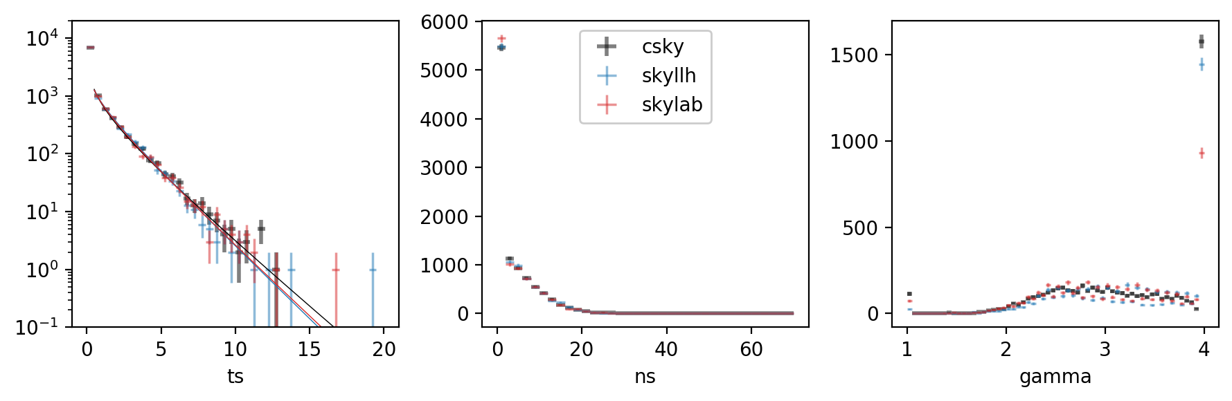
_images/99_csky_vs_skyllh_vs_skylab_54_0.png

The fits themselves came out like so:

[42]:

for (label,bg) in zip(labels,all_bgs):
    print('{:10} {}'.format(label, bg))

csky       Chi2TSD(10000 trials, eta=0.594, ndof=1.031, median=0.052 (from fit 0.046))
skyllh     Chi2TSD(10000 trials, eta=0.524, ndof=1.389, median=0.022 (from fit 0.019))
skylab     Chi2TSD(10000 trials, eta=0.536, ndof=1.283, median=0.023 (from fit 0.024))

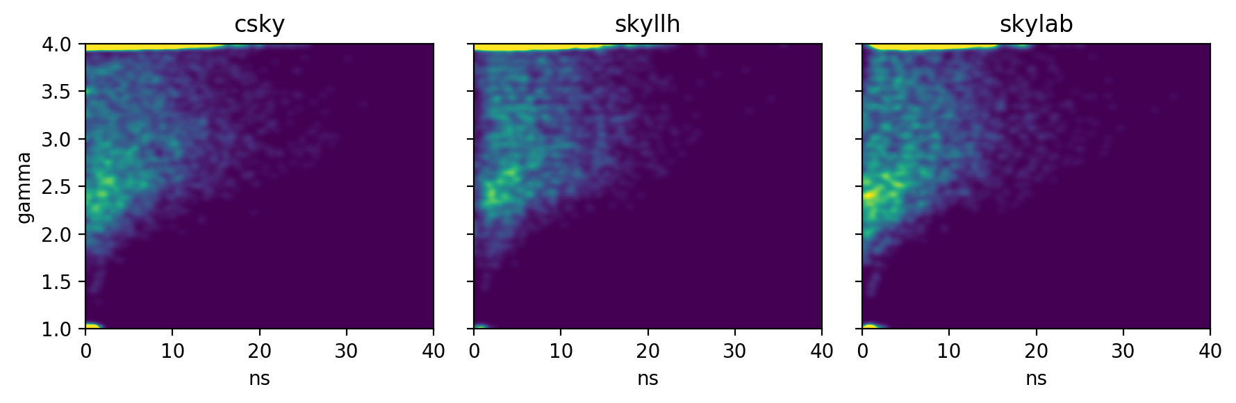
The \((n_s,\gamma)\) distributions are:

[43]:

fig, axs = plt.subplots(1, 3, figsize=(9,3), dpi=200, sharey=True)
for (b, label, ax) in zip(all_bgs, labels, axs):
    i = b.trials.ns > 0
    h = hl.hist((b.trials.ns[i], b.trials.gamma[i]),
                 bins=(np.r_[:40.01:1], np.r_[1:4.01:.1])).normalize()
    h = hl.kde((b.trials.ns[i], b.trials.gamma[i]), range=h.range)
    hl.plot2d(ax, h, vmax = 0.09, cmap='viridis')
    ax.set_title(label)
    ax.set_xlabel(r'ns')
axs[0].set_ylabel('gamma')
plt.tight_layout()

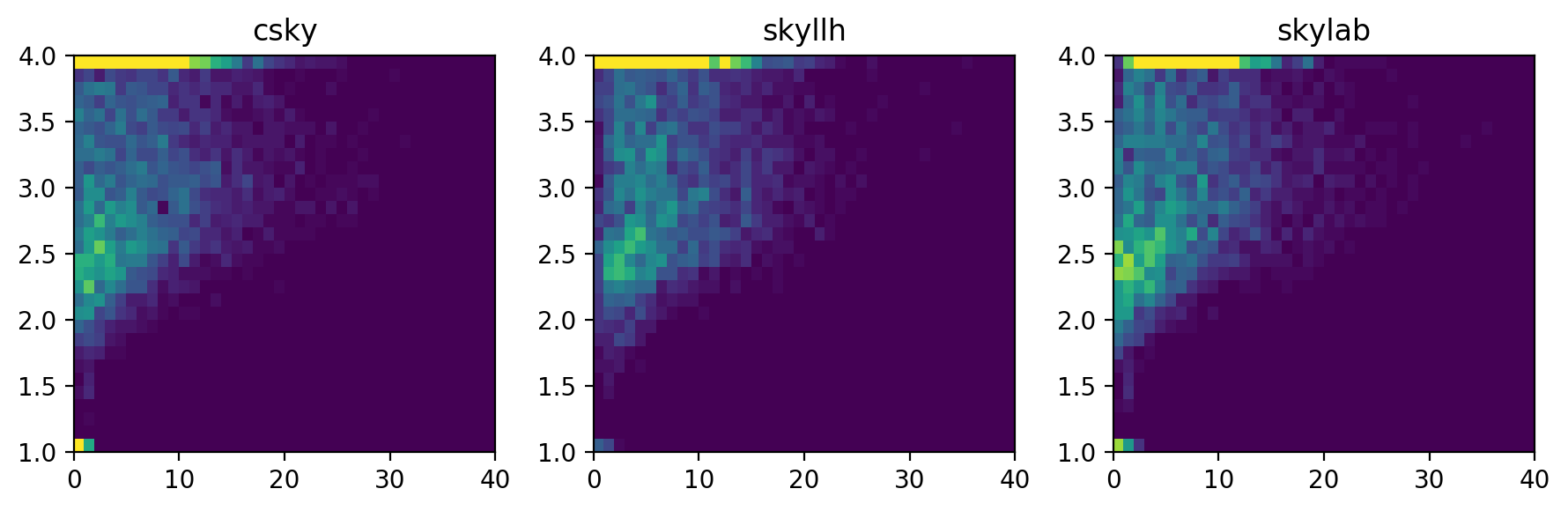
_images/99_csky_vs_skyllh_vs_skylab_58_0.png

or as raw histograms rather than KDE,

[44]:

fig, axs = plt.subplots(1, 3, figsize=(9,3), dpi=200)
for (b, label, ax) in zip(all_bgs, labels, axs):
    i = b.trials.ns > 0
    h = hl.hist((b.trials.ns[i], b.trials.gamma[i]),
                 bins=(np.r_[:40.01:1], np.r_[1:4.01:.1])).normalize()
    #h = hl.kde((b.trials.ns[i], b.trials.gamma[i]), range=h.range, kernel=(.02,.01))
    hl.plot2d(ax, h, vmax = 0.09, cmap='viridis')
    ax.set_title(label)
plt.tight_layout()

_images/99_csky_vs_skyllh_vs_skylab_60_0.png

Sensitivity estimation 

Sensitivity estimation can be done in a number of ways. csky provides an algorithm which performs an initial scan to identify the region of interest, and then performs batches of trials on a grid of signal strengths until the desired tolerance or maximum batch size is reached:

[30]:

timer = cy.timing.Timer()

[31]:

with timer.time('csky'):
    tr.find_n_sig(
        bg_csky.median(), 0.9, tol=.03,
        batch_size=1000, max_batch_size=1000, n_sig_step=1, mp_cpus=10)['n_sig']

Start time: 2019-07-25 12:26:57.631627
Using 10 cores.
* Starting initial scan for 90% of 50 trials with TS >= 0.052...
  n_sig = 1.000 ... frac = 0.68000
  n_sig = 2.000 ... frac = 0.74000
  n_sig = 3.000 ... frac = 0.78000
  n_sig = 4.000 ... frac = 0.92000
* Generating batches of 1000 trials...
n_trials | n_inj    0.00    1.60    3.20    4.80    6.40    8.00  |  n_sig(relative error)
1000     |         49.9%   73.3%   85.1%   92.0%   95.2%   98.2%  |      4.214 (+/-  4.7%) [spline]
End time: 2019-07-25 12:27:51.538601
Elapsed time: 0:00:53.906974

SkyLLH provides an algorithm that I haven’t fully understood yet – but given that it appears to run on a single core, the timing is potentially impressive:

[32]:

from skyllh.core.analysis_utils import estimate_sensitivity

[33]:

with timer.time('skyllh'):
    sens_skyllh = estimate_sensitivity(sana, rss, h0_ts_vals=skylab_10k_trials['ts'], eps_p=.03)

[==========================================================] 100% ELT 0h:00m:23s
[==========================================================] 100% ELT 0h:00m:21s
[==========================================================] 100% ELT 0h:00m:20s
[==========================================================] 100% ELT 0h:00m:19s
[==========================================================] 100% ELT 0h:00m:40s

[34]:

sens_skyllh

[34]:

(4.84375, 0.0)

Skylab provides an algorithm similar to that of csky:

[35]:

from skylab.sensitivity_utils import estimate_sensitivity as skylab_estimate_sensitivity

[36]:

with timer.time('skylab'):
    multillh.ncpu = 10
    skylab_sens = skylab_estimate_sensitivity(
        multillh, inj,
        src_ra=src_ra, src_dec=src_dec,
        ts_val=[bg_skylab.median(), 1], do_disc=False,
        ni_bounds=[0, 8])


Scanning injected event numbers [0.0, 8.0] ...
 [ 0] ni   0.00, TS   0.89, sigma  0.94 +/-  0.22 (20 trials/1.22 sec)
 [ 1] ni   1.60, TS   2.83, sigma  1.68 +/-  0.22 (20 trials/1.58 sec)
 [ 2] ni   3.20, TS   4.24, sigma  2.06 +/-  0.22 (20 trials/1.36 sec)
 [ 3] ni   4.80, TS   6.87, sigma  2.62 +/-  0.22 (20 trials/1.38 sec)
 [ 4] ni   6.40, TS   7.25, sigma  2.69 +/-  0.22 (20 trials/1.43 sec)
 [ 5] ni   8.00, TS  12.71, sigma  3.56 +/-  0.22 (20 trials/3.04 sec)

Initial Guesses ...
 Sensitivity ni   3.95, flux @ 1.0e+03 GeV is 3.27e-16 GeV^-1cm^-2s^-1
 Discovery   ni  13.18, flux @ 1.0e+03 GeV is 1.09e-15 GeV^-1cm^-2s^-1

Sensitivity Threshold ...
 Looking for 90% > Median TS (Median TS = 0.02)
 Scanning injected event range [0.00, 8.79]
 [ 0] ni  0.00, n  491, ntot 1000 (25.23 sec)
 [ 1] ni  1.76, n  739, ntot 1000 (31.81 sec)
 [ 2] ni  3.51, n  856, ntot 1000 (37.83 sec)
 [ 3] ni  5.27, n  935, ntot 1000 (36.75 sec)
 [ 4] ni  7.03, n  954, ntot 1000 (39.11 sec)
 [ 5] ni  8.79, n  980, ntot 1000 (43.94 sec)

Best fit:
  ndf -----------  4.05e+00 +/-  4.08e-01
  x0 ------------ -3.41e+00 +/-  4.87e-01
  reduced chi2 --  1.45 (dof 4)
  ni ------------  4.44 +/- 0.16 (p 0.90)
  flux ----------  3.67e-16 +/- 1.35e-17 GeV^-1cm^-2s^-1

[37]:

print(timer)

csky   | 0:00:53.908107
skyllh | 0:02:03.419458
skylab | 0:03:51.849178

Closing remarks 

We have compared the basic performance, results, and user experience of csky with SkyLLH and Skylab. Here are some conclusions:

Performance 

For our single core test, the csky:skyllh:skylab time elapsed ratio was 1:4.2025:4.7366. csky is clearly the fastest.
For our 10 core test, the timing ratio was similar.
The skyllh sensitivity estimation algorithm appears to be very fast.

Results 

The background TS, \(n_s\), \(\gamma\), and joint \((n_s,\gamma)\) distributions suggest that csky is better at fitting small signals, especially for spectra running into the limits \(\gamma\leq1\) or \(\gamma\geq4\). This may be due to its initial scan in \(\gamma\) prior to the full \((n_s,\gamma)\) fit.
csky also uses a denser default \(\gamma\) spacing of 0.0625, as opposed to 0.1. This naturally results in smoother \(\gamma\) distributions.
Otherwise the three libraries give good agreement on numerical results.

User experience 

Of course, the following are just one person’s (M. Richman) observations and opinions.

csky

Setup is extremely concise, not only for the single point source analysis tested here, but even for relatively complex likelihood and signal injection definitions.
Execution is the fastest out of tools tested.
Special-cased progress indicators appear for various stages: Analysis construction, trial generation, sensitivity estimation, [not shown here] skymap calculation.
Analysis cache-to-disk greatly reduces computational setup time.
Main advantage is probably the balance of flexibility and organic design. The PDF / signal acceptance / likelihood / minimizer framework was carefully thought out, but ultimately is small; specific use cases have been only one layer above this foundation, on an as-needed basis, and with C++ optimizations also added on an as-needed basis.

SkyLLH

Setup is relatively verbose, but if the user spells out the configuration herself, there can be no question what is the behavior of any aspect of the likelihood.
Execution is faster than skylab.
Generalized progress bars offer helpful estimate of estimated remaining time (but the user must consult the code to know what is happening, as no detailed feedback is given).
Analysis cache-to-disk would be very helpful in reducing setup time, but I don’t know if it is implemented.
Main advantage is probably the highly flexible design. The analysis you want to do might not already be implemented, but if it is not, then hopefully it is fairly obvious where the required pieces need to go.

Skylab

Amount of code required for setup is somewhat intermediate compared to csky or skyllh.
Execution is slowest of those tested, but profiling [not shown here] suggests that at least for time-integrated analysis, the main bottlenecks are necessary calculations: space and energy PDFs, minimizer iterations. It is to SkyLLH’s credit that it can run faster while maintaining the goals of numerical equivalence with skylab using pure python.
No feedback during trials.
Sensitivity estimation — I wish it could automatically deduce ni_bounds and wouldn’t make plots by default.
Multiprocessing for PointSourceLLH construction helps with setup time, but can’t beat cache-to-disk (which I believe is supposed to be possible with Skylab; I just don’t know how to do it).
Main advantage of Skylab is probably the amount of use and number of users it has had to date. For many analysis types, known-working examples are readily available.

Beyond these tests 

We’ve worked through the basics here, but there’s a lot more to cover, including:

all-sky scans (at least csky and Skylab have specialized tools for this)
time-dependent analysis (csky currently most flexible here so far)
spatial template analysis (csky can work with per-pixel spectra, or fit the spectrum for space-only templates)
spatial prior analysis (most developed in Skylab, basics mostly available in csky as well)
modified PDF constructions, e.g. joint space+energy (already available, I think, in SkyLLH)