Getting started with csky

In this tutorial, we’ll demonstrate how to get up and running with csky. The entire tutorial runs in about 15 minutes on my laptop (see timing summary at the bottom).

If not working on a cobalt, it’s easiest to get started if you set up a couple of environment variables. Here are the settings on my laptop:

export CSKY_DATA_ANALYSES_DIR="/home/mike/work/i3/data/analyses"
export CSKY_REMOTE_USER="mrichman"

You can confirm your own settings like so:

[3]:

import os
print(os.getenv('CSKY_DATA_ANALYSES_DIR'))
print(os.getenv('CSKY_REMOTE_USER'))

None
None

If you are working on a cobalt, you do not need to set these variables because you can read directly from the official data repositories.

Basic Setup 

We’ll import a few tools:

[4]:

import numpy as np
import matplotlib.pyplot as plt

import histlite as hl
import csky as cy

%matplotlib inline

I like to set up my plotting like so:

[5]:

cy.plotting.mrichman_mpl()

# for serif fonts:
# cy.plotting.mrichman_mpl(sans=False)

# for default rendering instead of LaTeX for everything
# cy.plotting.mrichman_mpl(tex=False)

/mnt/lfs7/user/ssclafani/software/external/csky/csky/plotting.py:92: MatplotlibDeprecationWarning: Support for setting the 'text.latex.preamble' or 'pgf.preamble' rcParam to a list of strings is deprecated since 3.3 and will be removed two minor releases later; set it to a single string instead.
  r'\SetSymbolFont{operators}   {sans}{OT1}{cmss} {m}{n}'

We’ll use a Timer to keep track of compute times:

[6]:

timer = cy.timing.Timer()
time = timer.time

For our first example, we’ll fire up an Analysis for the MESC-7yr dataset. csky works just as well for tracks, but cascades are nice for a tutorial because you can generate a reasonably accurate all-sky scan in just a minute or so. Below is what happens the first time you load the data on a non-cobalt machine. csky automatically fetches the required dataset files and stores them under $CSKY_DATA_ANALYSES_DIR.

[8]:

with time('ana setup (from scratch)'):
    ana = cy.get_analysis(cy.selections.Repository(), 'version-001-p02' , cy.selections.MESEDataSpecs.mesc_7yr)

Setting up Analysis for:
MESC_2010_2016
Setting up MESC_2010_2016...
Reading /data/ana/analyses/mese_cascades/version-001-p02/IC86_2013_MC.npy ...
Reading /data/ana/analyses/mese_cascades/version-001-p02/IC79_exp.npy ...
Reading /data/ana/analyses/mese_cascades/version-001-p02/IC86_2011_exp.npy ...
Reading /data/ana/analyses/mese_cascades/version-001-p02/IC86_2012_exp.npy ...
Reading /data/ana/analyses/mese_cascades/version-001-p02/IC86_2013_exp.npy ...
Reading /data/ana/analyses/mese_cascades/version-001-p02/IC86_2014_exp.npy ...
Reading /data/ana/analyses/mese_cascades/version-001-p02/IC86_2015_exp.npy ...
Reading /data/ana/analyses/mese_cascades/version-001-p02/IC86_2016_exp.npy ...
Reading /data/ana/analyses/mese_cascades/version-001-p02/GRL/IC79_exp.npy ...
Reading /data/ana/analyses/mese_cascades/version-001-p02/GRL/IC86_2011_exp.npy ...
Reading /data/ana/analyses/mese_cascades/version-001-p02/GRL/IC86_2012_exp.npy ...
Reading /data/ana/analyses/mese_cascades/version-001-p02/GRL/IC86_2013_exp.npy ...
Reading /data/ana/analyses/mese_cascades/version-001-p02/GRL/IC86_2014_exp.npy ...
Reading /data/ana/analyses/mese_cascades/version-001-p02/GRL/IC86_2015_exp.npy ...
Reading /data/ana/analyses/mese_cascades/version-001-p02/GRL/IC86_2016_exp.npy ...
Energy PDF Ratio Model...
  * gamma = 4.0000 ...
Signal Acceptance Model...
  * gamma = 4.0000 ...
Done.

0:00:08.400903 elapsed.

When you use a cy.selections.Repository to mirror files like this from within a notebook, you can check the stdout stream in the terminal where jupyter is running to monitor the download progress.

You are probably interested in tracks; here are some commonly used selections:

cy.selections.PSDataSpecs.ps_7yr – Stefan’s 7yr dataset
cy.selections.GFUDataSpecs.gfu_3yr – GFU subset used for TXS analysis
cy.selections.NTDataSpecs.nt_8yr – Northern tracks
cy.selections.PSDataSpecs.ps_10yr – Tessa’s 10yr dataset

We have used cy.selections.mrichman_repo here only because adding the cascade dataset to /data/ana/analyses is still TODO; for datasets already organized in the official repository, you can instead use cy.selections.repo to read from there.

Once you have an Analysis instance, you can cache it to disk:

[6]:

ana_dir = cy.utils.ensure_dir('/home/mike/work/i3/csky/ana')

[7]:

ana.save(ana_dir)

-> /home/mike/work/i3/csky/ana/MESC_2010_2016_DNN.subanalysis.npy

From now on, you can accelerate this setup step by reading from that directory (note that Repository objects also keep track of loaded files so they do not need to be re-loaded if used multiple times within the same session):

[8]:

with time('ana setup (from cache-to-disk)'):
    ana = cy.get_analysis(cy.selections.Repository(), 'version-001-p02', cy.selections.MESEDataSpecs.mesc_7yr, dir=ana_dir)

Setting up Analysis for:
MESC_2010_2016_DNN
Setting up MESC_2010_2016_DNN...
<- /home/mike/work/i3/csky/ana/MESC_2010_2016_DNN.subanalysis.npy
Done.

0:00:00.376400 elapsed.

csky’s “global” default configuration is stored as cy.CONF. By default it is just:

[9]:

print(cy.CONF)

{'mp_cpus': 1}

For the rest of the tutorial, we will be using this ana. We will also use 3 cores for multiprocessing-enabled steps (more can be appropriate, but this is a laptop).

[10]:

cy.CONF['ana'] = ana
cy.CONF['mp_cpus'] = 3

Point Source Analysis 

The hottest spot in my analysis was found at $(\alpha,\delta)=(271.23^\circ,7.78^\circ)$. Let’s get a trial runner for that position in the sky:

[11]:

src = cy.sources(271.23, 7.78, deg=True)
tr = cy.get_trial_runner(src=src)

cy.sources(ra,dec,**kw) is a convenience function for constructing cy.utils.Sources(**kw) instances. If ra and dec are arrays, then stacking analysis will be performed. If nonzero extension value(s) are given, Gaussian source extension is assumed.

cy.get_trial_runner(...) is a powerful function for obtaining cy.trial.TrialRunner instances. A trial runner is an object which is capable of working with “trials” (basically, event ensembles plus counts of “excluded” events pre-emptively counted as purely background, $S/B \to 0$). Trial runners not only produce trials, but also invoke likelihood fitting machinery for them; run them in (parallelizable) batches; and perform batches specifically useful for estimating sensitivities and discovery potentials. They also provide an interface for converting between event rates and fluxes/fluences.

Background estimation (PS)

The first step in most point source analyses is to characterize the background by running scrambled trials. In csky, this is done as follows:

[12]:

with time('ps bg trials'):
    n_trials = 10000
    bg = cy.dists.Chi2TSD(tr.get_many_fits(n_trials))

Performing 10000 background trials using 3 cores:
      10000/10000 trials complete.

0:00:34.311516 elapsed.

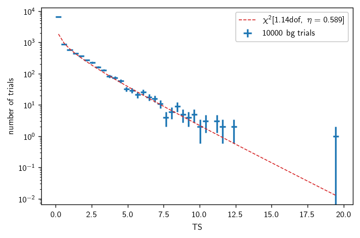
Chi2TSD stores the trials as well as a $\chi^2$ fit to the nonzero part of the TS distribution. We can look at a barebones summary:

[13]:

print(bg)

Chi2TSD(10000 trials, eta=0.589, ndof=1.140, median=0.058 (from fit 0.059))

or a more detailed one:

[14]:

print(bg.description)

Chi2TSD from 10000 trials:
           eta = 0.589
          ndof = 1.140
           loc = 0.000
         scale = 0.972
Thresholds from trials:
        median = 0.058
       1 sigma = 1.39
       2 sigma = 4.50
       3 sigma = 9.48
       4 sigma = 16.37
       5 sigma = 25.18
Thresholds from fit:
        median = 0.059
       1 sigma = 1.39
       2 sigma = 4.50
       3 sigma = 9.48
       4 sigma = 16.37
       5 sigma = 25.18

Finally, we can plot the distribution as follows:

[15]:

fig, ax = plt.subplots()

# csky uses histlite all over the place for PDF management
# the background distribution fit integrates with histlite as well
h = bg.get_hist(bins=50)
hl.plot1d(ax, h, crosses=True,
          label='{} bg trials'.format(bg.n_total))

# compare with the chi2 fit:
x = h.centers[0]
norm = h.integrate().values
ax.semilogy(x, norm * bg.pdf(x), lw=1, ls='--',
            label=r'$\chi^2[{:.2f}\text{{dof}},\ \eta={:.3f}]$'.format(bg.ndof, bg.eta))

# always label your plots, folks
ax.set_xlabel(r'TS')
ax.set_ylabel(r'number of trials')
ax.legend()
plt.tight_layout()

Sensitivity and discovery potential (PS)

We can estimate the sensitivity and discovery potential as follows:

[16]:

with time('ps sensitivity'):
    sens = tr.find_n_sig(
        # ts, threshold
        bg.median(),
        # beta, fraction of trials which should exceed the threshold
        0.9,
        # n_inj step size for initial scan
        n_sig_step=5,
        # this many trials at a time
        batch_size=500,
        # tolerance, as estimated relative error
        tol=.05
    )

Start time: 2019-09-26 10:41:14.457200
Using 3 cores.
* Starting initial scan for 90% of 50 trials with TS >= 0.058...
  n_sig = 5.000 ... frac = 0.84000
  n_sig = 10.000 ... frac = 0.96000
* Generating batches of 500 trials...
n_trials | n_inj    0.00    4.00    8.00   12.00   16.00   20.00  |  n_sig(relative error)
500      |         57.0%   86.8%   97.8%   99.0%  100.0%  100.0%  |      4.818 (+/-  6.8%) [spline]
1000     |         53.5%   84.6%   96.8%   99.2%  100.0%  100.0%  |      5.317 (+/-  3.7%) [spline]
End time: 2019-09-26 10:41:47.328998
Elapsed time: 0:00:32.871798

0:00:32.873298 elapsed.

[17]:

with time('ps discovery potential'):
    disc = tr.find_n_sig(bg.isf_nsigma(5), 0.5, n_sig_step=5, batch_size=500, tol=.05)

Start time: 2019-09-26 10:41:47.342592
Using 3 cores.
* Starting initial scan for 50% of 50 trials with TS >= 25.182...
  n_sig = 5.000 ... frac = 0.00000
  n_sig = 10.000 ... frac = 0.06000
  n_sig = 15.000 ... frac = 0.30000
  n_sig = 20.000 ... frac = 0.52000
* Generating batches of 500 trials...
n_trials | n_inj    0.00    8.00   16.00   24.00   32.00   40.00  |  n_sig(relative error)
500      |          0.0%    3.2%   31.8%   70.0%   96.2%  100.0%  |     19.787 (+/-  1.5%) [spline]
End time: 2019-09-26 10:42:06.300172
Elapsed time: 0:00:18.957580

0:00:18.963805 elapsed.

Now sens and disc are dict objects including various information about the calculation, as well as the result under the key n_sig:

[18]:

print(sens['n_sig'], disc['n_sig'])

5.316699361560448 19.786576686695103

So far, we’ve just found the Poisson event rates that correspond to the sensitivity and discovery potential fluxes. These can be converted to fluxes as follows:

[19]:

fmt = '{:.3e}  TeV/cm2/s @ 100 TeV'
# either the number of events or the whole dict will work
print(fmt.format(tr.to_E2dNdE(sens, E0=100, unit=1e3)))
print(fmt.format(tr.to_E2dNdE(disc['n_sig'], E0=100, unit=1e3)))

5.259e-12  TeV/cm2/s @ 100 TeV
1.957e-11  TeV/cm2/s @ 100 TeV

For more counts <–> flux conversions, see below.

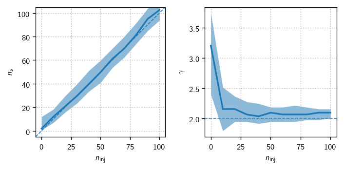
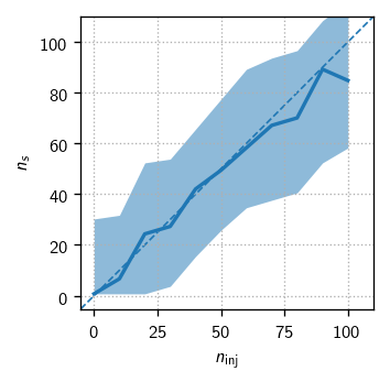
Test for fit bias (PS)

One powerful test of analysis readiness is to demonstrate that we can properly fit the parameters of an injected signal. For this we start by getting some batches of signal trials:

[20]:

n_sigs = np.r_[:101:10]
with time('ps fit bias trials'):
    trials = [tr.get_many_fits(100, n_sig=n_sig, logging=False, seed=n_sig) for n_sig in n_sigs]


0:00:11.244517 elapsed.

We add the true number of events injected for bookkeeping convenience:

[21]:

for (n_sig, t) in zip(n_sigs, trials):
    t['ntrue'] = np.repeat(n_sig, len(t))

Concatenate the trial batches:

[22]:

allt = cy.utils.Arrays.concatenate(trials)
allt

[22]:

Arrays(1100 items | columns: gamma, ns, ntrue, ts)

Finally, we make the plots:

[23]:

fig, axs = plt.subplots(1, 2, figsize=(6,3))

dns = np.mean(np.diff(n_sigs))
ns_bins = np.r_[n_sigs - 0.5*dns, n_sigs[-1] + 0.5*dns]
expect_kw = dict(color='C0', ls='--', lw=1, zorder=-10)
expect_gamma = tr.sig_injs[0].flux[0].gamma

ax = axs[0]
h = hl.hist((allt.ntrue, allt.ns), bins=(ns_bins, 100))
hl.plot1d(ax, h.contain_project(1),errorbands=True, drawstyle='default')

lim = ns_bins[[0, -1]]
ax.set_xlim(ax.set_ylim(lim))
ax.plot(lim, lim, **expect_kw)
ax.set_aspect('equal')


ax = axs[1]
h = hl.hist((allt.ntrue, allt.gamma), bins=(ns_bins, 100))
hl.plot1d(ax, h.contain_project(1),errorbands=True, drawstyle='default')
ax.axhline(expect_gamma, **expect_kw)
ax.set_xlim(axs[0].get_xlim())

for ax in axs:
    ax.set_xlabel(r'$n_\text{inj}$')
    ax.grid()
axs[0].set_ylabel(r'$n_s$')
axs[1].set_ylabel(r'$\gamma$')

plt.tight_layout()

Unblinding: confirming hottest spot 

Since this analysis is already unblinded, and paper submitted, in this tutorial we do not simulate the analysis review period and instead skip straight to unblinding!

[24]:

result = ts, ns, gamma = tr.get_one_fit(TRUTH=True)
print(result)

[9.143492673487607, 32.29657745559301, 2.9952804375887756]

We can view the result in a few different ways. For a nice table,

[25]:

print(tr.format_result(tr.get_one_fit(TRUTH=True)))

TS                  9.143492673487607
ns                  32.29657745559301
gamma               2.9952804375887756

For a more raw view, with named fit parameters rather than a flat array,

[26]:

tr.get_one_fit(TRUTH=True, flat=False)

[26]:

(9.143492673487607, {'gamma': 2.9952804375887756, 'ns': 32.29657745559301})

Finally, for full details including the complete minimizer configuration and convergence report,

[27]:

tr.get_one_fit(TRUTH=True, _full_output=True)

[27]:

(9.143492673487607,
 {'gamma': 2.9952804375887756, 'ns': 32.29657745559301},
 {},
 {'_full_output': True,
  '_ns_min': 0,
  '_ts_min': 0,
  '_ns_tol': 0.0001,
  '_taylor_tol': 0.001,
  '_fit_null': False,
  '_fmin_method': 'l_bfgs_b',
  '_fmin_factr': 1000000000.0,
  '_fmin_epsilon': 1e-08,
  '_seed_with_prior': True,
  '_seed_with_null': False,
  '_log_params': [],
  '_masks': None},
 {'grad': array([-1.24344979e-06]),
  'task': b'CONVERGENCE: NORM_OF_PROJECTED_GRADIENT_<=_PGTOL',
  'funcalls': 10,
  'nit': 3,
  'warnflag': 0})

We can also perform the fit with non-default parameters. For example, to constrain the spectral fit to $\gamma\in[1.5,2.5]$, seeding with $\gamma=2$, we can say:

[28]:

tr.get_one_fit(TRUTH=True, flat=False, gamma=[1.5, 2, 2.5])

[28]:

(6.519182178972011, {'gamma': 2.5, 'ns': 16.262526192118198})

We won’t do a thorough tour of the underlying objects performing these calculations, but let’s dig in only a little bit. A :class:LLHEvaluator instance is responsible for the actual fitting:

[29]:

L = tr.get_one_llh(TRUTH=True)
L.fit(**tr.fitter_args)

[29]:

(9.143492673487607, {'gamma': 2.9952804375887756, 'ns': 32.29657745559301})

We can also take a look at the trial data itself:

[30]:

trial = tr.get_one_trial(TRUTH=True) # event ensemble and count of masked-out events
print(trial)
L = tr.get_one_llh_from_trial(trial)
L.fit(**tr.fitter_args)

Trial(evss=[[Events(1875 items | columns: dec, idx, inj, log10energy, ra, sigma, sindec)]], n_exs=[104])

[30]:

(9.143492673487607, {'gamma': 2.9952804375887756, 'ns': 32.29657745559301})

Ok, now finally, we use the pre-computed bg to calculate the p-value:

[31]:

print('p = {:.2e} ({:.2f} sigma)'.format(bg.sf(ts), bg.sf_nsigma(ts)))

p = 1.63e-03 (2.94 sigma)

In my paper draft, I claim 2.8 sigma based on a whole lot more trials.

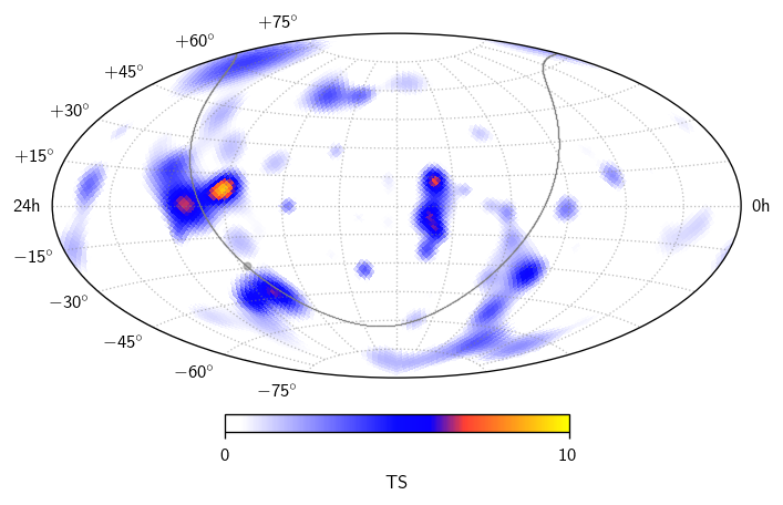
All-sky scan 

In many analyses, we aren’t just interested in specific sky coordinates, but instead a scan over the whole sky. In csky we can do this using a cy.trial.SkyScanTrialRunner, obtained like so:

[32]:

sstr = cy.get_sky_scan_trial_runner(mp_scan_cpus=3, nside=32)

[33]:

with time('ps all-sky scan'):
    scan = sstr.get_one_scan(TRUTH=True, logging=True)

Scanning 12288 locations using 3 cores:
      12288/12288 coordinates complete.

0:00:33.151653 elapsed.

What do we have here?

[34]:

scan.shape

[34]:

(4, 12288)

The second axis is npix for the selected healpy nside. The first axis has items $(-\log_{10}(p),\text{TS},n_s,\gamma)$. In this example we haven’t bothered to characterize the background in detail, so the scan[0] is simply a copy of scan[1]. To obtain proper p-values, pass an argument get_sky_scan_trial_runner(..., ts_to_p=[function]), where [function] should accept dec[radians],ts and return p, typically by using cy.dists.ts_to_p.

We can plot the TS map like so:

[35]:

fig, ax = plt.subplots (subplot_kw=dict (projection='aitoff'))
sp = cy.plotting.SkyPlotter(pc_kw=dict(cmap=cy.plotting.skymap_cmap, vmin=0, vmax=10))
mesh, cb = sp.plot_map(ax, scan[1], n_ticks=2)
kw = dict(color='.5', alpha=.5)
sp.plot_gp(ax, lw=.5, **kw)
sp.plot_gc(ax, **kw)
ax.grid(**kw)
cb.set_label(r'TS')
plt.tight_layout()

Galactic Plane 

csky provides two types of template analysis: space-only templates, and per-pixel energy-binned spectra. In the former, more common type, we provide a space-only healpix map describing the signal distribution across the sky. My mrichman_repo provides the Fermi-LAT $\pi^0$-decay template:

[36]:

pi0_map = cy.selections.mrichman_repo.get_template ('Fermi-LAT_pi0_map')

Reading /home/mike/work/i3/data/analyses/templates/Fermi-LAT_pi0_map.npy ...

The desired template analysis can be expressed as a configuration dict, which will ultimately be overlayed on top of cy.CONF:

[37]:

pi0_conf = {
    # desired template
    'template': pi0_map,
    # desired baseline spectrum
    'flux':     cy.hyp.PowerLawFlux(2.5),
    # desired fixed spectrum in likelihood
    'fitter_args': dict(gamma=2.5),
    # use signal subtracting likelihood
    'sigsub': True,
    # fastest construction:
    # weight from acceptance parameterization rather
    # than pixel-by-pixel directly from MC
    'fast_weight': True,
    # cache angular-resolution-smeared maps to disk
    'dir': cy.utils.ensure_dir('{}/templates/pi0'.format(ana_dir))
}

[38]:

with time('pi0 template construction'):
    pi0_tr = cy.get_trial_runner(pi0_conf)

MESC_2010_2016_DNN        | Acceptance weighting complete.
MESC_2010_2016_DNN        | Smearing complete.
-> /home/mike/work/i3/csky/ana/templates/pi0/MESC_2010_2016_DNN.template.fastweight.npy

0:00:14.135515 elapsed.

mrichman_repo also provides the KRAγ templates:

[39]:

krag5_map, krag5_energy_bins = cy.selections.mrichman_repo.get_template(
    'KRA-gamma_5PeV_maps_energies', per_pixel_flux=True)

Reading /home/mike/work/i3/data/analyses/templates/KRA-gamma_5PeV_maps_energies.tuple.npy ...

[40]:

krag5_conf = {
    'template': krag5_map,
    'bins_energy': krag5_energy_bins,
    'fitter_args': dict(gamma=2.5),
    'update_bg' : True,
    'sigsub': True,
    'dir': cy.utils.ensure_dir('{}/templates/kra'.format(ana_dir))}

[42]:

with time('KRAγ5 template construction'):
    krag5_tr = cy.get_trial_runner(krag5_conf)

MESC_2010_2016_DNN        | Acceptance weighting complete.
MESC_2010_2016_DNN        | Smearing complete.
-> /home/mike/work/i3/csky/ana/templates/kra/MESC_2010_2016_DNN.template.npy

0:00:26.555365 elapsed.

As we will see, all the usual trial runner functionality is available.

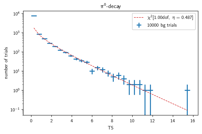
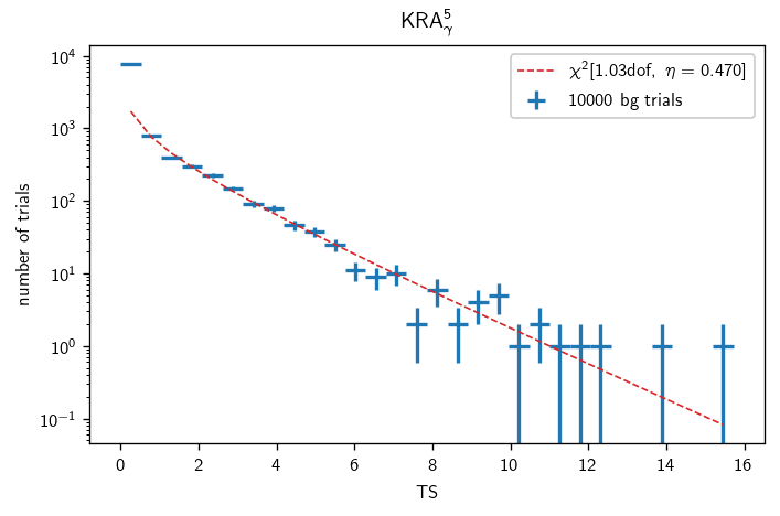
Background characterization (GP)

[43]:

with time('pi0 bg trials'):
    n_trials = 10000
    pi0_bg = cy.dists.Chi2TSD(pi0_tr.get_many_fits(n_trials))

Performing 10000 background trials using 3 cores:
      10000/10000 trials complete.

0:00:28.301643 elapsed.

[44]:

with time('KRAγ5 bg trials'):
    n_trials = 10000
    krag5_bg = cy.dists.Chi2TSD(krag5_tr.get_many_fits(n_trials))

Performing 10000 background trials using 3 cores:
      10000/10000 trials complete.

0:00:11.343195 elapsed.

[45]:

bgs = pi0_bg, krag5_bg
titles = '$\pi^0$-decay', 'KRA$_\gamma^5$'
for (b, title) in zip(bgs, titles):
    fig, ax = plt.subplots()
    h = b.get_hist(bins=30)
    hl.plot1d(ax, h, crosses=True,
              label='{} bg trials'.format(bg.n_total))
    x = h.centers[0]
    norm = h.integrate().values
    ax.semilogy(x, norm * b.pdf(x), lw=1, ls='--',
                label=r'$\chi^2[{:.2f}\text{{dof}},\ \eta={:.3f}]$'.format(b.ndof, b.eta))
    ax.set_xlabel(r'TS')
    ax.set_ylabel(r'number of trials')
    ax.set_title(title)
    ax.legend()
    plt.tight_layout()

Sensitivity and discovery potential (GP)

We’ll find the sensitivity and discovery potential the same way as we did above for a point source:

[46]:

with time('pi0 sensitivity'):
    pi0_sens = pi0_tr.find_n_sig(pi0_bg.median(), 0.9, n_sig_step=10, batch_size=500, tol=.05)

Start time: 2019-09-26 10:44:26.457045
Using 3 cores.
* Starting initial scan for 90% of 50 trials with TS >= 0.000...
  n_sig = 10.000 ... frac = 0.56000
  n_sig = 20.000 ... frac = 0.78000
  n_sig = 30.000 ... frac = 0.86000
  n_sig = 40.000 ... frac = 0.98000
* Generating batches of 500 trials...
n_trials | n_inj    0.00   16.00   32.00   48.00   64.00   80.00  |  n_sig(relative error)
500      |         44.6%   78.2%   90.2%   97.2%   99.4%   99.8%  |     31.639 (+/-  6.6%) [spline]
1000     |         46.6%   75.2%   88.5%   96.8%   99.5%   99.7%  |     34.347 (+/-  3.5%) [spline]
End time: 2019-09-26 10:47:24.457213
Elapsed time: 0:02:58.000168

0:02:58.001318 elapsed.

[47]:

with time('pi0 discovery potential'):
    pi0_disc = pi0_tr.find_n_sig(pi0_bg.isf_nsigma(5), 0.5, n_sig_step=20, batch_size=500, tol=.05)

Start time: 2019-09-26 10:47:24.467355
Using 3 cores.
* Starting initial scan for 50% of 50 trials with TS >= 24.101...
  n_sig = 20.000 ... frac = 0.00000
  n_sig = 40.000 ... frac = 0.00000
  n_sig = 60.000 ... frac = 0.00000
  n_sig = 80.000 ... frac = 0.00000
  n_sig = 100.000 ... frac = 0.08000
  n_sig = 120.000 ... frac = 0.22000
  n_sig = 140.000 ... frac = 0.40000
  n_sig = 160.000 ... frac = 0.58000
* Generating batches of 500 trials...
n_trials | n_inj    0.00   64.00  128.00  192.00  256.00  320.00  |  n_sig(relative error)
500      |          0.0%    0.8%   32.4%   84.4%   94.6%   96.6%  |    148.888 (+/-  1.1%) [spline]
End time: 2019-09-26 10:49:08.611245
Elapsed time: 0:01:44.143890

0:01:44.146194 elapsed.

[48]:

with time('KRAγ5 sensitivity'):
    krag5_sens = krag5_tr.find_n_sig(krag5_bg.median(), 0.9, n_sig_step=10, batch_size=500, tol=.05)

Start time: 2019-09-26 10:49:08.618539
Using 3 cores.
* Starting initial scan for 90% of 50 trials with TS >= 0.000...
  n_sig = 10.000 ... frac = 0.70000
  n_sig = 20.000 ... frac = 0.88000
  n_sig = 30.000 ... frac = 0.98000
* Generating batches of 500 trials...
n_trials | n_inj    0.00   12.00   24.00   36.00   48.00   60.00  |  n_sig(relative error)
500      |         47.8%   76.0%   91.8%   98.6%   99.8%  100.0%  |     22.002 (+/-  6.2%) [spline]
1000     |         48.1%   78.1%   92.1%   97.9%   99.8%  100.0%  |     21.373 (+/-  4.1%) [spline]
End time: 2019-09-26 10:53:05.232254
Elapsed time: 0:03:56.613715

0:03:56.615738 elapsed.

[49]:

with time('KRAγ5 discovery potential'):
    krag5_disc = krag5_tr.find_n_sig(krag5_bg.isf_nsigma(5), 0.5, n_sig_step=20, batch_size=500, tol=.05)

Start time: 2019-09-26 10:53:05.244537
Using 3 cores.
* Starting initial scan for 50% of 50 trials with TS >= 23.837...
  n_sig = 20.000 ... frac = 0.00000
  n_sig = 40.000 ... frac = 0.00000
  n_sig = 60.000 ... frac = 0.18000
  n_sig = 80.000 ... frac = 0.34000
  n_sig = 100.000 ... frac = 0.74000
* Generating batches of 500 trials...
n_trials | n_inj    0.00   40.00   80.00  120.00  160.00  200.00  |  n_sig(relative error)
500      |          0.0%    0.8%   39.8%   91.6%   99.6%  100.0%  |     87.707 (+/-  1.6%) [spline]
End time: 2019-09-26 10:55:17.222720
Elapsed time: 0:02:11.978183

0:02:11.981155 elapsed.

[50]:

print('pi0-decay sens/disc:')
print(fmt.format(pi0_tr.to_E2dNdE(pi0_sens, E0=100, unit=1e3)))
print(fmt.format(pi0_tr.to_E2dNdE(pi0_disc, E0=100, unit=1e3)))

pi0-decay sens/disc:
2.340e-11  TeV/cm2/s @ 100 TeV
1.014e-10  TeV/cm2/s @ 100 TeV

[51]:

print('KRAγ5 sens/disc:')
print('{} x KRAγ5'.format(krag5_tr.to_model_norm(krag5_sens, E0=100, unit=1e3)))
print('{} x KRAγ5'.format(krag5_tr.to_model_norm(krag5_disc, E0=100, unit=1e3)))

KRAγ5 sens/disc:
0.581590224006752 x KRAγ5
2.386635444613829 x KRAγ5

Test for fit bias (π⁰)

Once again, we’ll follow the pattern from the PS analysis described above.

[52]:

with time('pi0 fit bias trials'):
    pi0_trials = [pi0_tr.get_many_fits(100, n_sig=n_sig, logging=False, seed=n_sig) for n_sig in n_sigs]


0:00:37.967059 elapsed.

[53]:

for (n_sig, t) in zip(n_sigs, pi0_trials):
    t['ntrue'] = np.repeat(n_sig, len(t))

[54]:

allt = cy.utils.Arrays.concatenate(pi0_trials)
allt

[54]:

Arrays(1100 items | columns: ns, ntrue, ts)

[55]:

fig, ax = plt.subplots(1, figsize=(3,3))

dns = np.mean(np.diff(n_sigs))
ns_bins = np.r_[n_sigs - 0.5*dns, n_sigs[-1] + 0.5*dns]
expect_kw = dict(color='C0', ls='--', lw=1, zorder=-10)
expect_gamma = tr.sig_injs[0].flux[0].gamma

h = hl.hist((allt.ntrue, allt.ns), bins=(ns_bins, 100))
hl.plot1d(ax, h.contain_project(1),errorbands=True, drawstyle='default')

lim = 1.05 * ns_bins[[0, -1]]
ax.set_xlim(ax.set_ylim(lim))
ax.plot(lim, lim, **expect_kw)
ax.set_aspect('equal')

ax.set_xlabel(r'$n_\text{inj}$')
ax.grid()
ax.set_ylabel(r'$n_s$')

plt.tight_layout()

Unblinding (GP)

Finally, we obtain the unblinded result:

[56]:

pi0_result = pi0_tr.get_one_fit(TRUTH=True)
print(pi0_tr.format_result(pi0_result))

TS                  3.0484314194823994
ns                  44.68690065047474

[57]:

pi0_ts = pi0_result[0]
print('p = {:.2e} ({:.2f} sigma)'.format(pi0_bg.sf(pi0_ts), pi0_bg.sf_nsigma(pi0_ts)))

p = 3.70e-02 (1.79 sigma)

[58]:

krag5_result = krag5_tr.get_one_fit(TRUTH=True)
print(krag5_tr.format_result(krag5_result))

TS                  4.055486117489724
ns                  31.091825690526317

[59]:

krag5_ts = krag5_result[0]
print('p = {:.2e} ({:.2f} sigma)'.format(krag5_bg.sf(krag5_ts), krag5_bg.sf_nsigma(krag5_ts)))

p = 1.92e-02 (2.07 sigma)

In the paper draft, I claim p=0.040 and p=0.021 respectively, again based on a whole lot more trials.

Counts <–> flux conversions 

Counts <–> flux conversions can be pretty error prone; csky tries to make them easy. Here are a few examples, assuming for now that ns from the all-sky hottest spot actually corresponds to an $E^{-2}$ spectrum:

[60]:

tr.to_dNdE(ns) # 1/GeV/cm2/s  @  1 GeV

[60]:

3.1945011757861e-08

[61]:

tr.to_dNdE(ns, E0=1e5) # 1/GeV/cm2/s  @  10^5 GeV

[61]:

3.1945011757861e-18

[62]:

tr.to_E2dNdE(ns, E0=1e5) # GeV/cm2/s  @  10^5 GeV

[62]:

3.1945011757861e-08

[63]:

tr.to_E2dNdE(ns, E0=100, unit=1e3) # TeV/cm2/s  @  100 TeV

[63]:

3.1945011757861e-11

But it was actually a different spectrum right?

[64]:

print('all-sky hottest spot TS, ns, gamma = {}, {}, {}'.format(ts, ns, gamma))

all-sky hottest spot TS, ns, gamma = 9.143492673487607, 32.29657745559301, 2.9952804375887756

We can convert to a flux for that spectrum too:

[65]:

tr.to_E2dNdE(ns, gamma=gamma, E0=100, unit=1e3) # TeV/cm2/s  @  100 TeV, for gamma ~ 3.002

[65]:

6.4612895507279714e-12

Of course, any of these flux values can be converted back to event rates:

[66]:

tr.to_ns(6.46128955072804e-12, gamma=gamma, E0=100, unit=1e3)

[66]:

32.29657745559335

Timing summary 

[67]:

print(timer)

ana setup (from scratch)       | 0:00:19.693964
ana setup (from cache-to-disk) | 0:00:00.376400
ps bg trials                   | 0:00:34.311516
ps sensitivity                 | 0:00:32.873298
ps discovery potential         | 0:00:18.963805
ps fit bias trials             | 0:00:11.244517
ps all-sky scan                | 0:00:33.151653
pi0 template construction      | 0:00:14.135515
KRAγ5 template construction    | 0:00:26.555365
pi0 bg trials                  | 0:00:28.301643
KRAγ5 bg trials                | 0:00:11.343195
pi0 sensitivity                | 0:02:58.001318
pi0 discovery potential        | 0:01:44.146194
KRAγ5 sensitivity              | 0:03:56.615738
KRAγ5 discovery potential      | 0:02:11.981155
pi0 fit bias trials            | 0:00:37.967059
-----------------------------------------------
total                          | 0:15:19.662335

Closing remarks 

In this tutorial, we’ve just scratched the surface of what you can do with csky. I hope I’ve convinced you that it’s easy, fast, and maybe even fun.

What now? Try it yourself, ask questions, and consult the other tutorials and documentation.