Correlated analyses with MultiTrialRunner

In this tutorial, we consider the use case of multiple, potentially partially-correlated analyses. Here, we want to perform multiple likelihood tests on the same “trials” — the same realizations of the datasets.

import numpy as np
import matplotlib.pyplot as plt

import histlite as hl
import csky as cy

%matplotlib inline

cy.plotting.mrichman_mpl()

/mnt/lfs7/user/ssclafani/software/external/csky/csky/plotting.py:92: MatplotlibDeprecationWarning: Support for setting the 'text.latex.preamble' or 'pgf.preamble' rcParam to a list of strings is deprecated since 3.3 and will be removed two minor releases later; set it to a single string instead.
  r'\SetSymbolFont{operators}   {sans}{OT1}{cmss} {m}{n}'

ana_dir = '/data/user/mrichman/csky_cache/ana'

We’ll test with one year of data, PS IC86-2011.

ana = cy.get_analysis(cy.selections.repo, 'version-003-p02' , cy.selections.PSDataSpecs.ps_2011, dir=ana_dir)

Setting up Analysis for:
IC86_2011
Setting up IC86_2011...
Reading /data/ana/analyses/ps_tracks/version-003-p02/IC86_2011_MC.npy ...
Reading /data/ana/analyses/ps_tracks/version-003-p02/IC86_2011_exp.npy ...
Reading /data/ana/analyses/ps_tracks/version-003-p02/GRL/IC86_2011_exp.npy ...
<- /data/user/mrichman/csky_cache/ana/IC86_2011.subanalysis.version-003-p02.npy
Done.

Everything that follows will use this same Analysis, so we put it in cy.CONF.

cy.CONF['ana'] = ana
cy.CONF['mp_cpus'] = 15

Individual Trial Runners

We begin by setting up an arbitrary catalog of two sources:

ra = np.r_[0, 180]
dec = np.r_[-45, 45]
src = cy.sources(ra, dec, deg=True)
src.as_dataframe

	dec	dec_deg	sindec	ra	ra_deg	weight	extension	extension_deg
0	-0.785398	-45.0	-0.707107	0.000000	0.0	0.5	0.0	0.0
1	0.785398	45.0	0.707107	3.141593	180.0	0.5	0.0	0.0

We get a trial runner for each:

trs = [cy.get_trial_runner(src=s) for s in src]
trs

[<csky.trial.TrialRunner at 0x7f91d37d5080>,
 <csky.trial.TrialRunner at 0x7f91baf133c8>]

Now for the tricky part: we need to make sure our background trials have events for every source, but we don’t want to scramble the whole sky. So we set up our “injection” trial runner to know about the whole catalog.

We also need to decide on how the signal injection should work; here we’ll just inject signals for the 0th source.

tr_inj = cy.get_trial_runner(src=src, inj_conf=dict(src=src[0]))

To confirm that signal events wind up where they should, let’s look at an example trial:

trial = tr_inj.get_one_trial(n_sig=5, poisson=False, seed=2)
trial

Trial(evss=[[Events(13188 items | columns: dec, idx, inj, log10energy, ra, sigma, sindec), Events(5 items | columns: dec, idx, inj, log10energy, ra, sigma, sindec)]], n_exs=[123056])

trial.evss[0][1].as_dataframe

	dec	log10energy	ra	sigma	sindec	idx	inj
0	-0.789157	5.577282	0.000794	0.003491	-0.704913	773766	<csky.inj.PointSourceInjector object at 0x7f91...
1	-0.831554	5.118237	0.008226	0.011637	-0.736841	311727	<csky.inj.PointSourceInjector object at 0x7f91...
2	-0.787004	5.241669	0.003833	0.003491	-0.720210	698751	<csky.inj.PointSourceInjector object at 0x7f91...
3	-0.789060	5.397988	0.001629	0.005621	-0.702275	499808	<csky.inj.PointSourceInjector object at 0x7f91...
4	-0.773355	5.275870	6.279155	0.018069	-0.697965	746488	<csky.inj.PointSourceInjector object at 0x7f91...

As you can see, the signal events have ra,dec where they should.

Background trials

In order to get per-test p-values, we need to run background trials for each source. At this step, correlations between tests do not matter, so we can still use the ordinary trial runners.

%time bgs = [cy.dists.Chi2TSD(tr.get_many_fits(1e3)) for tr in trs]
bgs

Performing 1000 background trials using 15 cores:
       1000/1000 trials complete.
Performing 1000 background trials using 15 cores:
       1000/1000 trials complete.
CPU times: user 422 ms, sys: 225 ms, total: 646 ms
Wall time: 4.65 s

[Chi2TSD(1000 trials, eta=0.503, ndof=1.105, median=0.000 (from fit 0.000)),
 Chi2TSD(1000 trials, eta=0.540, ndof=1.060, median=0.013 (from fit 0.013))]

MultiTrialRunner

We are ready to perform “simultaneous” trials for all hypothesis tests. For this we use a MultiTrialRunner.

multr = cy.trial.MultiTrialRunner(
    # the Analysis
    ana,
    # bg+sig injection trial runner (produces trials)
    tr_inj,
    # llh test trial runners (perform fits given trials)
    trs,
    # background distrubutions
    bgs=bgs,
    # use multiprocessing
    mp_cpus=cy.CONF['mp_cpus'],
)

One more time without interspersed comments:

multr = cy.trial.MultiTrialRunner(ana, tr_inj, trs, bgs=bgs, mp_cpus=cy.CONF['mp_cpus'])

Single Trial

A single trial looks like so:

trial_kw = dict(n_sig=10, poisson=False, seed=2)
multr.get_one_fit(**trial_kw)

array([ 8.39466146, 32.19708837, 10.61458083,  2.06225432,  0.26760624,
        0.        ,  0.        ,  3.        ])

This output is easier to understand if you make this call, which breaks up the result per-source:

multr.get_all_fits(**trial_kw)

[array([ 8.39466146, 32.19708837, 10.61458083,  2.06225432]),
 array([0.26760624, 0.        , 0.        , 3.        ])]

No we can see what’s happening: for each source, we get mlog10p,ts,ns,gamma, or \((-\log_{10}(p),\text{TS},n_s,\gamma)\). Since we’ve injected lots of signal for the 0th source, the significance is over 5σ:

from scipy import stats
stats.norm.isf(10**-7.633)

5.463963905200207

Note that technically, the bgs argument was optional. If we don’t provide it, then as a fallback we get “fake” mlog10p which just duplicate TS:

multr_nobg = cy.trial.MultiTrialRunner(ana, tr_inj, trs)
multr_nobg.get_all_fits(**trial_kw)

[array([32.19708837, 32.19708837, 10.61458083,  2.06225432]),
 array([0., 0., 0., 3.])]

MultiTrialRunner trials

We’re ready to perform a batch of trials using MultiTrialRunner.

trials = multr.get_many_fits(1000, n_sig=10, seed=1)

Performing 1000 trials with n_sig = 10.000 using 15 cores:
       1000/1000 trials complete.

trials

Arrays(1000 items | columns: gamma_0000, gamma_0001, mlog10p_0000, mlog10p_0001, ns_0000, ns_0001, ts_0000, ts_0001)

The results have been tabulated according to the name of the fit parameters and indices of the sources. Let’s look at the results for the first few trials:

trials.as_dataframe.head()

	gamma_0000	gamma_0001	mlog10p_0000	mlog10p_0001	ns_0000	ns_0001	ts_0000	ts_0001
0	1.972629	3.250000	10.400346	0.267606	14.934783	0.000000	40.814930	0.000000
1	2.028484	4.000000	7.719988	0.267606	13.135672	0.000000	29.309175	0.000000
2	2.075980	2.842599	4.350988	0.335503	8.785978	0.919642	15.035911	0.046768
3	1.923978	4.000000	9.293134	0.267606	13.924785	0.000000	36.052241	0.000000
4	2.025977	2.000000	5.080775	0.267606	7.943536	0.000000	18.098095	0.000000

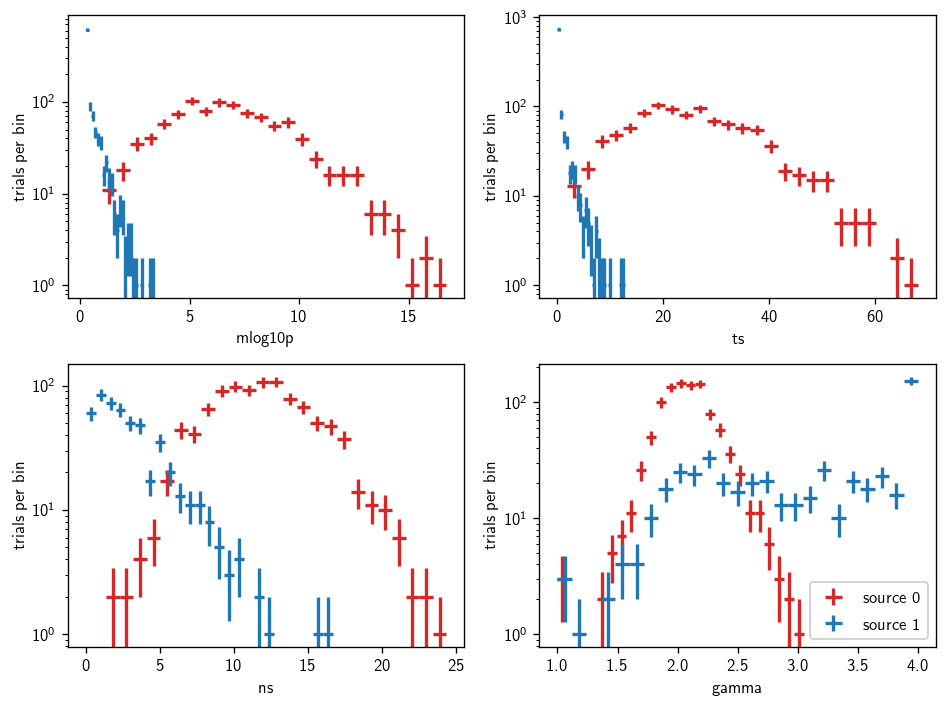
Once again, since we’ve injected plenty of signal (10 events per trial, but now with Poisson smearing), we see that the results are much more significant for source 0000 than for source 0001 (which only has background nearby).

We can plot the resulting distributions like so:

fig, axs = plt.subplots(2, 2, figsize=(8,6))
axs = np.ravel(axs)
names = 'mlog10p ts ns gamma'.split()
for (i, name) in enumerate(names):
    ax = axs[i]
    mask0 = trials.ns_0000 > 0 if name in 'ns gamma' else trials.ns_0000 >= 0
    mask1 = trials.ns_0001 > 0 if name in 'ns gamma' else trials.ns_0001 >= 0
    hl.plot1d(ax, hl.hist(trials[name+'_0000'][mask0], bins=25), crosses=True, color='C1', label='source 0')
    hl.plot1d(ax, hl.hist(trials[name+'_0001'][mask1], bins=25), crosses=True, color='C0', label='source 1')
    ax.set_xlabel(name)
    ax.set_ylabel(r'trials per bin')
    ax.semilogy()
ax.legend()
plt.tight_layout()

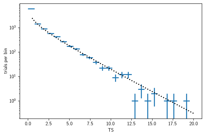
Stacking

The simplest way to implement a stacking analysis is to simply add the TS values. Let’s do some background trials for that setup:

bg_trials = multr.get_many_fits(10e3, seed=1)
bg_trials['sum_ts'] = np.sum([bg_trials[name] for name in bg_trials.keys() if 'ts' in name], axis=0)

Performing 10000 background trials using 15 cores:
      10000/10000 trials complete.

sum_bg = cy.dists.Chi2TSD(bg_trials.sum_ts)

fig, ax = plt.subplots()
h = sum_bg.get_hist(bins=25)
hl.plot1d(ax, h, crosses=True)
norm = h.integrate().values
x = np.linspace(.5, 20, 300)
ax.plot(x, norm * sum_bg.pdf(x), 'k:')
ax.set_xlabel(r'TS')
ax.set_ylabel(r'trials per bin')
ax.semilogy()
plt.tight_layout()

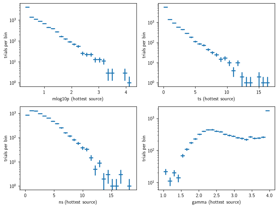
Hottest source analysis

We might be interested in the hottest source in each trial. Then the “post-trials” test statistic is just the maximum mlog10p from each trial. This can be obtained like so:

mlog10p = np.array([bg_trials[name] for name in bg_trials.keys() if name.startswith('mlog10p_')])
ts = np.array([bg_trials[name] for name in bg_trials.keys() if name.startswith('ts_')])
ns = np.array([bg_trials[name] for name in bg_trials.keys() if name.startswith('ns_')])
gamma = np.array([bg_trials[name] for name in bg_trials.keys() if name.startswith('gamma_')])

imax = np.argmax(mlog10p, axis=0)
r = np.arange(len(imax))
bg_trials_hottest = cy.utils.Arrays(dict(
    mlog10p=mlog10p[imax,r], ts=ts[imax,r], ns=ns[imax,r], gamma=gamma[imax,r]))

fig, axs = plt.subplots(2, 2, figsize=(8,6))
axs = np.ravel(axs)
names = 'mlog10p ts ns gamma'.split()
for (i, name) in enumerate(names):
    ax = axs[i]
    mask = bg_trials_hottest.ns > 0 if name in 'ns gamma' else bg_trials_hottest.ns >= 0
    hl.plot1d(ax, hl.hist(bg_trials_hottest[name][mask], bins=25), crosses=True)
    ax.set_xlabel(name + ' (hottest source)')
    ax.set_ylabel(r'trials per bin')
    ax.semilogy()
plt.tight_layout()

p-values from single batch

Above we described the most intuitive way to set all this up. Technically, the initial trial batches may be redundant if equal statistics are required for the per-hypothesis background distributions and the final distributions used for post-trials calculations.

We can do all the work with one batch; let’s see how. First we run some trials:

%time t = multr_nobg.get_many_fits(10000, seed=1, mp_cpus=15)

Performing 10000 background trials using 15 cores:
      10000/10000 trials complete.
CPU times: user 52.9 ms, sys: 149 ms, total: 202 ms
Wall time: 12.2 s

t.as_dataframe.head()

	gamma_0000	gamma_0001	mlog10p_0000	mlog10p_0001	ns_0000	ns_0001	ts_0000	ts_0001
0	3.250000	3.250000	0.000000	0.000000	0.000000	0.000000	0.000000	0.000000
1	4.000000	4.000000	4.938129	0.000000	5.184195	0.000000	4.938129	0.000000
2	3.236252	2.842487	0.030601	0.046903	0.332028	0.921009	0.030601	0.046903
3	2.043473	4.000000	1.255303	0.000000	2.614685	0.000000	1.255303	0.000000
4	2.500000	2.000000	0.000000	0.000000	0.000000	0.000000	0.000000	0.000000

We fit each TS distribution:

new_bgs = [cy.dists.Chi2TSD(t['ts_{:04d}'.format(i)]) for i in range(len(src))]
new_bgs

[Chi2TSD(10000 trials, eta=0.524, ndof=1.119, median=0.005 (from fit 0.007)),
 Chi2TSD(10000 trials, eta=0.500, ndof=1.016, median=0.000 (from fit 0.000))]

And finally, we patch the mlog10p values:

for i in range(len(src)):
    suffix = '_{:04d}'.format(i)
    t['mlog10p'+suffix] = -np.log10(new_bgs[i].sf(t['ts'+suffix]))

t.as_dataframe.head()

	gamma_0000	gamma_0001	mlog10p_0000	mlog10p_0001	ns_0000	ns_0001	ts_0000	ts_0001
0	3.250000	3.250000	0.280752	0.300596	0.000000	0.000000	0.000000	0.000000
1	4.000000	4.000000	1.741344	0.300596	5.184195	0.000000	4.938129	0.000000
2	3.236252	2.842487	0.329330	0.371563	0.332028	0.921009	0.030601	0.046903
3	2.043473	4.000000	0.795645	0.300596	2.614685	0.000000	1.255303	0.000000
4	2.500000	2.000000	0.280752	0.300596	0.000000	0.000000	0.000000	0.000000

Remarks

Here we’ve demonstrated how to perform an analysis that includes multiple hypothesis tests. In general, one can either:

• Characterize the background for each hypothesis test, independently:

• Run more trials using a MultiTrialRunner so that correlations between hypothesis tests are properly accounted for.

Or:

• Run trials with a MultiTrialRunner and, if needed, compute per-test p-values from distributions fitted to those trials.

Either way, MultiTrialRunner provides a mechanism for efficiently performing trials that account for possible partial correlations between multiple hypothesis tests.