TXS 0506+056 time-integrated and time-dependent

In this tutorial, we’ll reproduce some TXS 0506+056 results.

Setup 

[1]:

import numpy as np
import matplotlib.pyplot as plt
from scipy import stats

import histlite as hl
import csky as cy

%matplotlib inline

[2]:

cy.plotting.mrichman_mpl()

We’ll set up a timer:

[3]:

timer = cy.timing.Timer()
time = timer.time

Let’s grab the “PS + GFU” sample, using version-002-p01 for each, and disabling the angular error floor (which was not included in the original analysis):

[4]:

ana_dir = cy.utils.ensure_dir('/data/user/mrichman/csky_cache/ana')

[5]:

with time('ana setup'):
    ana = cy.get_analysis(
        cy.selections.repo,
        'version-002-p01', cy.selections.PSDataSpecs.ps_7yr,
        'version-002-p01', cy.selections.GFUDataSpecs.gfu_3yr,
        dir=ana_dir, min_sigma=0)

Setting up Analysis for:
IC40, IC59, IC79, IC86_2011, IC86_2012_2014, GFU_2015_2017
Setting up IC40...
Reading /data/ana/analyses/ps_tracks/version-002-p01/IC40_corrected_MC.npy ...
Reading /data/ana/analyses/ps_tracks/version-002-p01/IC40_exp.npy ...
Reading /data/ana/analyses/ps_tracks/version-002-p01/IC40_GRL.npy ...
<- /data/user/mrichman/csky_cache/ana/IC40.subanalysis.version-002-p01.npy
Setting up IC59...
Reading /data/ana/analyses/ps_tracks/version-002-p01/IC59_corrected_MC.npy ...
Reading /data/ana/analyses/ps_tracks/version-002-p01/IC59_exp.npy ...
Reading /data/ana/analyses/ps_tracks/version-002-p01/IC59_GRL.npy ...
<- /data/user/mrichman/csky_cache/ana/IC59.subanalysis.version-002-p01.npy
Setting up IC79...
Reading /data/ana/analyses/ps_tracks/version-002-p01/IC79b_corrected_MC.npy ...
Reading /data/ana/analyses/ps_tracks/version-002-p01/IC79b_exp.npy ...
Reading /data/ana/analyses/ps_tracks/version-002-p01/IC79b_GRL.npy ...
<- /data/user/mrichman/csky_cache/ana/IC79.subanalysis.version-002-p01.npy
Setting up IC86_2011...
Reading /data/ana/analyses/ps_tracks/version-002-p01/IC86_corrected_MC.npy ...
Reading /data/ana/analyses/ps_tracks/version-002-p01/IC86_exp.npy ...
Reading /data/ana/analyses/ps_tracks/version-002-p01/IC86_GRL.npy ...
<- /data/user/mrichman/csky_cache/ana/IC86_2011.subanalysis.version-002-p01.npy
Setting up IC86_2012_2014...
Reading /data/ana/analyses/ps_tracks/version-002-p01/IC86-2012_corrected_MC_v2.npy ...
Reading /data/ana/analyses/ps_tracks/version-002-p01/IC86-2012_exp_v2.npy ...
Reading /data/ana/analyses/ps_tracks/version-002-p01/IC86-2013_exp_v2.npy ...
Reading /data/ana/analyses/ps_tracks/version-002-p01/IC86-2014_exp_v2.npy ...
Reading /data/ana/analyses/ps_tracks/version-002-p01/IC86-2012_GRL.npy ...
Reading /data/ana/analyses/ps_tracks/version-002-p01/IC86-2013_GRL.npy ...
Reading /data/ana/analyses/ps_tracks/version-002-p01/IC86-2014_GRL.npy ...
<- /data/user/mrichman/csky_cache/ana/IC86_2012_2014.subanalysis.version-002-p01.npy
Setting up GFU_2015_2017...
Reading /data/ana/analyses/gfu/version-002-p01/SplineMPEmax.MuEx.MC.npy ...
Reading /data/ana/analyses/gfu/version-002-p01/SplineMPEmax.MuEx.IC86-2015.npy ...
Reading /data/ana/analyses/gfu/version-002-p01/SplineMPEmax.MuEx.IC86-2016.npy ...
Reading /data/ana/analyses/gfu/version-002-p01/SplineMPEmax.MuEx.IC86-2017.npy ...
Reading /data/ana/analyses/gfu/version-002-p01/SplineMPEmax.MuEx.GRL.npy ...
<- /data/user/mrichman/csky_cache/ana/GFU_2015_2017.subanalysis.version-002-p01.npy
Done.

0:00:52.551711 elapsed.

We’ll also look at the 2012-2014 configuration alone:

[6]:

with time('ana_12_14 setup'):
    ana_12_14 = cy.get_analysis(
        cy.selections.repo,
        'version-002-p01', cy.selections.PSDataSpecs.ps_7yr[-1],
        dir=ana_dir, min_sigma=0)

Setting up Analysis for:
IC86_2012_2014
Setting up IC86_2012_2014...
<- /data/user/mrichman/csky_cache/ana/IC86_2012_2014.subanalysis.version-002-p01.npy
Done.

0:00:02.544739 elapsed.

From here on, we’ll use ana and mp_cpus=10 wherever relevant, unless otherwise specified:

[7]:

cy.CONF['ana'] = ana
cy.CONF['mp_cpus'] = 10

Time-integrated analysis 

We can grab the coordinates from a (currently very short) list of pre-defined sources:

[8]:

src = cy.sources(*cy.selections.Coordinates.txs_0506_056[:2])
cy.CONF['src'] = src

We construct the single-source trial runner:

[9]:

tr = cy.get_trial_runner()

Here’s the result:

[10]:

with time('unblind time integrated'):
    print(tr.get_one_fit(TRUTH=True, flat=False))

(18.663818740946425, {'gamma': 2.0291608496153426, 'ns': 15.332733637279862})

0:00:00.083892 elapsed.

We should also check the p-value.

[11]:

with time('bg trials time integrated'):
    bg = cy.dists.Chi2TSD(tr.get_many_fits(1000, seed=1))

Performing 1000 background trials using 10 cores:
       1000/1000 trials complete.

0:00:09.737622 elapsed.

[12]:

bg.sf_nsigma(tr.get_one_fit(TRUTH=True)[0])

[12]:

4.05949407168683

We know that in practice more background scrambles are required to really pin down a significance at this level, but this is pretty close to the accepted value.

Untriggered single flare — Gaussian 

Here’s the untriggered Gaussian single-flare fit for 2012-2014:

[13]:

conf_gauss = {
    'time': 'utf',
    'seeder': cy.seeding.UTFSeeder(),
    'fitter_args': dict(_log_params='dt', _fmin_method='minuit'),
    'concat_evs': True
}
tr_gauss = cy.get_trial_runner(conf_gauss, ana=ana_12_14)
tr_gauss_ps_gfu = cy.get_trial_runner(conf_gauss, ana=ana)

[14]:

with time('unblind gaussian flare'):
    print(tr_gauss.format_result(tr_gauss.get_one_fit(TRUTH=True)))

TS                  23.136275598269947
ns                  13.046011428453836
t0                  57006.184382641426
dt                  54.8228829919159
gamma               2.1318043821995247

0:00:00.801333 elapsed.

This is similar to, though not exactly the same as, the official result. We get better agreement with the original result (from psLab) if we disable detailed accounting for the GRL (in the signal time PDF):

[15]:

with time('unblind gaussian flare'):
    print(tr_gauss.format_result(tr_gauss.get_one_fit(TRUTH=True, use_grl=False)))

TS                  22.023591770597093
ns                  12.577074639465641
t0                  57004.84556952451
dt                  55.534056983245726
gamma               2.1167311263655715

0:00:00.559732 elapsed.

We find the same flare in a full PS+GFU (i.e. multi-dataset) analysis:

[16]:

with time('unblind gaussian flare (ps+gfu)'):
    print(tr_gauss_ps_gfu.format_result(tr_gauss_ps_gfu.get_one_fit(TRUTH=True)))

TS                  20.796921427881177
ns                  13.030879169522892
t0                  57005.575320121075
dt                  53.82572764881969
gamma               2.1315463983861895

0:00:19.714746 elapsed.

Note that to_E2dNdE, etc., return fluences rather than fluxes for time-dependent analyses:

[17]:

fit_params = tr_gauss.get_one_fit(TRUTH=True, flat=False)[1]
print('{:.3e} TeV/cm2'.format(tr_gauss.to_E2dNdE(E0=100, unit=1e3, **fit_params)))
fit_params = tr_gauss.get_one_fit(TRUTH=True, flat=False, use_grl=False)[1]
print('{:.3e} TeV/cm2 (neglecting GRL)'.format(tr_gauss.to_E2dNdE(E0=100, unit=1e3, **fit_params)))

2.155e-04 TeV/cm2
2.108e-04 TeV/cm2 (neglecting GRL)

Let’s check the p-value:

[18]:

with time('bg trials gaussian flare'):
    bg_gauss = cy.dists.Chi2TSD(tr_gauss.get_many_fits(1000, seed=1))

Performing 1000 background trials using 10 cores:
       1000/1000 trials complete.

0:01:06.775784 elapsed.

[19]:

bg_gauss.sf(22.67), bg_gauss.sf_nsigma(22.67)

[19]:

(5.8009972504182815e-05, 3.8543870175381363)

To match the official result, we need a trial factor 9.5yr/3yr:

[20]:

stats.norm.isf(bg_gauss.sf(22.67) * 9.5/3)

[20]:

3.5624595771843457

Next, let’s use a SkyScanTrialRunner to map out the region nearby region:

[21]:

RA, DEC = cy.trial.SkyScanTrialRunner.get_rectangular_grid(
    src.ra[0], src.dec[0], np.radians(6), np.radians(2/2**3))
sstr = cy.get_sky_scan_trial_runner(conf_gauss, src=src, ana=ana_12_14, scan_ra=RA, scan_dec=DEC)

[22]:

with time('sky scan gaussian flare'):
    scan = sstr.get_one_scan(TRUTH=True, mp_cpus=10, logging=True)

Scanning 625 locations using 10 cores:
        625/625 coordinates complete.

0:00:41.679475 elapsed.

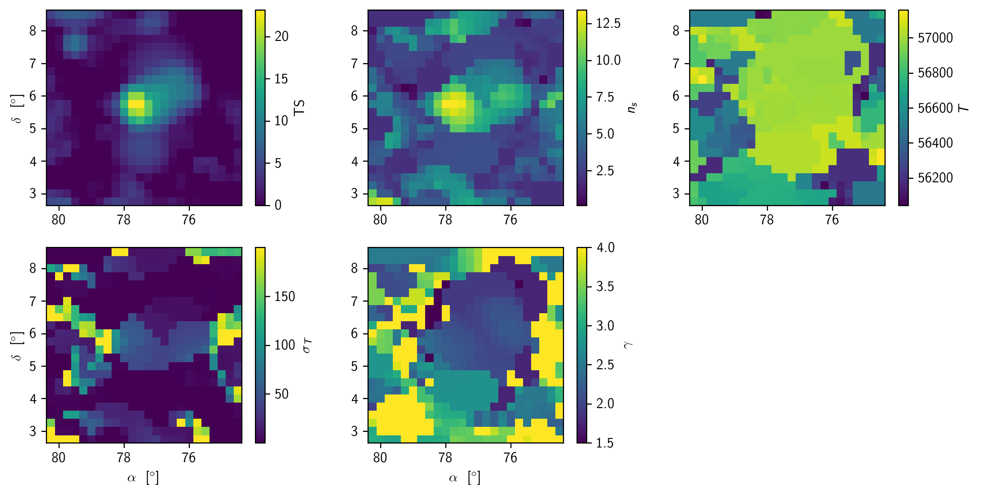
Here are plots of the best fit:

[23]:

fig, oaxs = plt.subplots(2, 3, figsize=(10,5), dpi=200)
axs = np.ravel(oaxs)
labels = r'TS $n_s$ $T$ $\sigma_T$ $\gamma$'.split()
for (i, (ax, m)) in enumerate(zip(axs, scan[1:])):
    pc = ax.pcolormesh(np.degrees(RA), np.degrees(DEC), m)
    cb = fig.colorbar(pc, ax=ax)
    cb.set_label(labels[i])
    ax.set_xlim(ax.get_xlim()[::-1])
    ax.set_aspect('equal')
for ax in oaxs[-1]:
    ax.set_xlabel(r'$\alpha\ \ [^\circ]$')
for ax in oaxs[:,0]:
    ax.set_ylabel(r'$\delta\ \ [^\circ]$')
axs[-1].set_visible(False)
plt.tight_layout()

Untriggered single flare — step function 

By default, untriggered flare analysis fits a Gaussian signal time PDF. We can also perform a box-window search:

[24]:

conf_box = {
    'time': 'utf',
    'box': True,
    'seeder': cy.seeding.UTFSeeder(),
}

[25]:

tr_box = cy.get_trial_runner(conf_box, ana=ana_12_14)

[26]:

with time('unblind box flare'):
    print(tr_box.format_result(tr_box.get_one_fit(TRUTH=True)))

TS                  28.48249947602982
ns                  13.45388195814707
t0                  57013.62927017009
dt                  151.6205902344591
gamma               2.158717128472718

0:00:00.865713 elapsed.

[27]:

fit_params = tr_box.get_one_fit(TRUTH=True, flat=False)[1]
print('{:.3e} TeV/cm2'.format(tr_box.to_E2dNdE(E0=100, unit=1e3, **fit_params)))

2.150e-04 TeV/cm2

This is slightly different from the official result, though the specific reasons have not yet been determined. According to our implementation, this really is a slightly better fit than the official result:

[28]:

print(tr_box.get_one_fit(TRUTH=True, t0=57004+13, dt=159, seeder=None, flat=False))

(28.354866951770635, {'gamma': 2.1846017881006956, 'ns': 13.992756991949692})

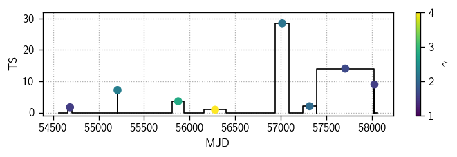
Multiflare 

multiflare analysis was recently added to csky. For this we get a MultiflareTrialRunner:

[29]:

mtr = cy.get_multiflare_trial_runner(src=src, ana=ana, max_dt=2000)

[30]:

with time('unblind multiflare'):
    result_multiflare = mtr.get_one_fit(TRUTH=True, logging=True)

    3 /     3 ... 0:00:00.013713 elapsed.
  378 /   378 ... 0:00:01.559281 elapsed.
   36 /    36 ... 0:00:00.075493 elapsed.
  105 /   105 ... 0:00:00.290528 elapsed.
 1275 /  1275 ... 0:00:04.851777 elapsed.
 2278 /  2278 ... 0:00:10.272435 elapsed.

0:00:17.267262 elapsed.

[31]:

print(mtr.format_result(result_multiflare))

ts                  66.96751539769558
ns_total            41.32806989887902
gamma_mean          2.2522205167780407
ts_no_prior         101.13580074401915
n_flare             8
n_flare_tested      4075
Flares(
    src, TS, ns, gamma, TS0 =   0,  28.482,  13.45, 2.16  32.37 | [56937.818975 -> 57089.439565] ( 151.620590)
    src, TS, ns, gamma, TS0 =   0,  14.041,   3.27, 1.67  14.73 | [57391.443843 -> 58018.871186] ( 627.427342)
    src, TS, ns, gamma, TS0 =   0,   8.973,   1.36, 1.55  17.87 | [58018.871186 -> 58029.256078] (  10.384892)
    src, TS, ns, gamma, TS0 =   0,   7.188,   4.27, 2.27  15.16 | [55204.982082 -> 55211.545663] (   6.563581)
    src, TS, ns, gamma, TS0 =   0,   3.607,   7.23, 2.81   5.49 | [55808.334098 -> 55938.004387] ( 129.670289)
    src, TS, ns, gamma, TS0 =   0,   2.041,   3.21, 2.03   5.52 | [57236.013093 -> 57391.443843] ( 155.430751)
    src, TS, ns, gamma, TS0 =   0,   1.706,   1.54, 1.53   6.11 | [54666.328255 -> 54707.987934] (  41.659679)
    src, TS, ns, gamma, TS0 =   0,   0.929,   6.99, 4.00   3.88 | [56156.855129 -> 56398.468652] ( 241.613523)
)

We can plot the neutrino “lightcurve” like so:

[32]:

lc = result_multiflare[-1]

[33]:

fig, ax = plt.subplots(figsize=(6,2))
hts = lc.to_hist('ts')
hl.plot1d(ax, hts, color='k', lw=1)
hgamma = lc.to_hist('gamma')
m = hts.values > 0
sc = ax.scatter(hts.centers[0][m], hts.values[m], c=hgamma.values[m], vmin=1, vmax=4, zorder=10)
cb = fig.colorbar(sc)
cb.set_label(r'$\gamma$')
ax.set_xlabel(r'MJD')
ax.set_ylabel(r'TS')
ax.set_ylim(-1,32)
ax.grid()
plt.tight_layout()

Timing summary 

[34]:

print(timer)

ana setup                       | 0:00:52.551711
ana_12_14 setup                 | 0:00:02.544739
unblind time integrated         | 0:00:00.083892
bg trials time integrated       | 0:00:09.737622
unblind gaussian flare          | 0:00:00.559732
unblind gaussian flare (ps+gfu) | 0:00:19.714746
bg trials gaussian flare        | 0:01:06.775784
sky scan gaussian flare         | 0:00:41.679475
unblind box flare               | 0:00:00.865713
unblind multiflare              | 0:00:17.267262
------------------------------------------------
total                           | 0:03:31.780676

Remarks 

The results above are not identical to the official results. Here is a summary of known differences and their explanations:

Time-integrated: In the official results, no-longer-recommended settings were used in the energy PDF ratio construction: namely, the so-called “skylab” (as opposed to “classic”) method of filling empty bins in the background energy PDF, and rectangular-kernel smoothing of the energy PDFs. Those settings induce some undesireable biases. Here, we do not reproduce those settings, and thus the results are slightly different.
Gaussian flare: The central time of the best-fit flare obtained here is slightly different than the one originally obtained. This may be due to slightly different settings originally used in pslab, which so far does not (as far as I know) use GRL details in the signal time PDF; nor does it bin the energy or background space PDFs in a way that necessarily matches the standard used in csky, Skylab, and SkyLLH.
Box flare: Again we obtain a result similar, though not identical, to the official result.
Multiflare: Thanks to detailed investigations by W. Luszczak, csky’s multiflare implementation appears to be reliable and ready for use. Here we recover to good precision the result he originally obtained with Skylab.

TXS 0506+056 time-integrated and time-dependent

Setup

Time-integrated analysis

Untriggered single flare — Gaussian

Untriggered single flare — step function

Multiflare

Timing summary

Remarks