Differential Sensitivity
In this tutorial, we’ll compute a differential sensitivity.
Setup
[2]:
import numpy as np
import matplotlib.pyplot as plt

import histlite as hl
import csky as cy

%matplotlib inline
[3]:
cy.plotting.mrichman_mpl()
/home/mkovacevich/updated_csky_2/csky/csky/plotting.py:92: MatplotlibDeprecationWarning: Support for setting the 'text.latex.preamble' or 'pgf.preamble' rcParam to a list of strings is deprecated since 3.3 and will be removed two minor releases later; set it to a single string instead.
  r'\SetSymbolFont{operators}   {sans}{OT1}{cmss} {m}{n}'
[4]:
timer = cy.timing.Timer()
time = timer.time
We’ll work with MESC 7yr because things are fast with a low-stats dataset.
[5]:
with time('ana setup'):
    ana = cy.get_analysis(cy.selections.repo, cy.selections.MESEDataSpecs.mesc_7yr)
Setting up Analysis for:
MESC_2010_2016
Setting up MESC_2010_2016...
Reading /data/ana/analyses/mese_cascades/version-001-p02/IC86_2013_MC.npy ...
Reading /data/ana/analyses/mese_cascades/version-001-p02/IC79_exp.npy ...
Reading /data/ana/analyses/mese_cascades/version-001-p02/IC86_2011_exp.npy ...
Reading /data/ana/analyses/mese_cascades/version-001-p02/IC86_2012_exp.npy ...
Reading /data/ana/analyses/mese_cascades/version-001-p02/IC86_2013_exp.npy ...
Reading /data/ana/analyses/mese_cascades/version-001-p02/IC86_2014_exp.npy ...
Reading /data/ana/analyses/mese_cascades/version-001-p02/IC86_2015_exp.npy ...
Reading /data/ana/analyses/mese_cascades/version-001-p02/IC86_2016_exp.npy ...
Reading /data/ana/analyses/mese_cascades/version-001-p02/GRL/IC79_exp.npy ...
Reading /data/ana/analyses/mese_cascades/version-001-p02/GRL/IC86_2011_exp.npy ...
Reading /data/ana/analyses/mese_cascades/version-001-p02/GRL/IC86_2012_exp.npy ...
Reading /data/ana/analyses/mese_cascades/version-001-p02/GRL/IC86_2013_exp.npy ...
Reading /data/ana/analyses/mese_cascades/version-001-p02/GRL/IC86_2014_exp.npy ...
Reading /data/ana/analyses/mese_cascades/version-001-p02/GRL/IC86_2015_exp.npy ...
Reading /data/ana/analyses/mese_cascades/version-001-p02/GRL/IC86_2016_exp.npy ...
Energy PDF Ratio Model...
  * gamma = 4.0000 ...
Signal Acceptance Model...
  * gamma = 4.0000 ...
Done.

0:00:11.353483 elapsed.
And we’ll examine \(\delta=-60^\circ\) so that we can compare the results with pre-unblinding calculations here.
[6]:
src = cy.sources(0, -60, deg=True)
Background estimation
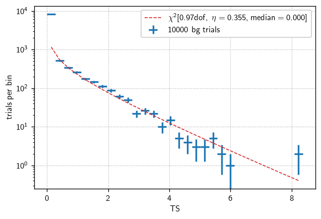
In IceCube analyses, when we refer to differential sensitivity, we are talking about the sensitivity to signal events in relatively narrow energy bands. Just like ordinary (all-energy, or energy-integrated) sensitivity calculations, we’re looking for the flux that yields greater than the background-only median TS in 90% of trials.
Therefore, we start by finding the background-only TS distribution and extracting that median value.
[7]:
with time('background estimation'):
    allE_tr = cy.get_trial_runner(ana=ana, src=src)
    bg = cy.dists.Chi2TSD(allE_tr.get_many_fits(10000, mp_cpus=10))
Performing 10000 background trials using 10 cores:
      10000/10000 trials complete.

0:00:11.512436 elapsed.
[12]:
fig, ax = plt.subplots()

#The warning indicates that a bin is empty
h = bg.get_hist(bins=30)
hl.plot1d(ax, h, crosses=True,
          label='{} bg trials'.format(bg.n_total))

x = h.centers[0]
norm = h.integrate().values
ax.semilogy(x, norm * bg.pdf(x), lw=1, ls='--',
            label=r'$\chi^2[{:.2f}\text{{dof}},\ \eta={:.3f}, \text{{median}}={:.3f}]$'.format(
                bg.ndof, bg.eta, bg.median()))

ax.set(xlabel='TS', ylabel='trials per bin')
ax.legend()
ax.grid()
/home/mkovacevich/new_venv/lib/python3.7/site-packages/numpy/core/_asarray.py:102: UserWarning: Warning: converting a masked element to nan.
  return array(a, dtype, copy=False, order=order)
Differential Sensitivity
Now we are ready for the main calculation. We start by defining energy bins and corresponding trial runners:
[13]:
# you could also use np.logspace()
Ebins = 10**np.r_[3:7.1:.25]
trs = [
    cy.get_trial_runner(
        ana=ana, src=src,
        flux=cy.hyp.PowerLawFlux(2, energy_range=(Emin, Emax)))
    for (Emin, Emax) in zip(Ebins[:-1], Ebins[1:])
]
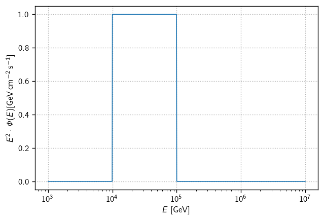
Notice the energy_range argument here. This defines a flux that is zero except for within the given range (which is always specified in GeV to match the true_energy values in our MC). To drive the point home, consider a flux defined in the energy range 10-100 TeV:
[14]:
flux = cy.hyp.PowerLawFlux(2, energy_range=(1e4, 1e5))

fig, ax = plt.subplots()
E = np.logspace(3, 7, 1000)
ax.semilogx(E, E**2 * flux(E), lw=1)
ax.set(
    xlabel=r'$E$ [GeV]',
    ylabel=r'$E^2\cdot\Phi(E) [\text{GeV}\,\text{cm}^{-2}\,\text{s}^{-1}]$',
)
ax.grid()
The sensitivity can be computed in the usual way with tr.find_n_sig(). However, to convert to a flux we must be careful to evaluate at an E0 where the flux is nonzero. Otherwise, where \(\Phi(E_0)\) appears in the n \(\to\) flux conversion, the flux will evaluate to zero.
[15]:
senss = []

with time('differential sensitivity'):
    for (Emin, Emax, tr) in zip(Ebins[:-1], Ebins[1:], trs):
        print(f'log10(E) bin: {np.log10(Emin), np.log10(Emax)}')
        sens = tr.find_n_sig(
            bg.median(), .9,
            n_sig_start=5, n_sig_step=10, batch_size=500, max_batch_size=500,
            seed=1, mp_cpus=10)
        # N.B. must set E0 to a value within the energy_range
        # of the flux for this trial runner
        sens['E2dNdE'] = tr.to_E2dNdE(sens, E0=Emin)
        senss.append(sens)
log10(E) bin: (3.0, 3.25)
Start time: 2021-07-28 13:52:12.259510
Using 10 cores.
* Starting initial scan for 90% of 50 trials with TS >= 0.000...
  n_sig = 5.000 ... frac = 0.44000
  n_sig = 15.000 ... frac = 0.52000
  n_sig = 25.000 ... frac = 0.44000
  n_sig = 35.000 ... frac = 0.70000
  n_sig = 45.000 ... frac = 0.78000
  n_sig = 55.000 ... frac = 0.96000
* Generating batches of 500 trials...
n_trials | n_inj    0.00   22.00   44.00   66.00   88.00  110.00  |  n_sig(relative error)
500      |         33.2%   51.6%   81.0%   94.6%   99.6%  100.0%  |     56.278 (+/-  3.0%) [spline]
End time: 2021-07-28 13:52:24.277669
Elapsed time: 0:00:12.018159
log10(E) bin: (3.25, 3.5)
Start time: 2021-07-28 13:52:24.280796
Using 10 cores.
* Starting initial scan for 90% of 50 trials with TS >= 0.000...
  n_sig = 5.000 ... frac = 0.48000
  n_sig = 15.000 ... frac = 0.84000
  n_sig = 25.000 ... frac = 0.88000
  n_sig = 35.000 ... frac = 0.96000
* Generating batches of 500 trials...
n_trials | n_inj    0.00   14.00   28.00   42.00   56.00   70.00  |  n_sig(relative error)
500      |         37.0%   70.8%   95.0%   99.4%   99.8%  100.0%  |     23.511 (+/-  2.9%) [spline]
End time: 2021-07-28 13:52:35.519420
Elapsed time: 0:00:11.238624
log10(E) bin: (3.5, 3.75)
Start time: 2021-07-28 13:52:35.523987
Using 10 cores.
* Starting initial scan for 90% of 50 trials with TS >= 0.000...
  n_sig = 5.000 ... frac = 0.58000
  n_sig = 15.000 ... frac = 0.92000
* Generating batches of 500 trials...
n_trials | n_inj    0.00    6.00   12.00   18.00   24.00   30.00  |  n_sig(relative error)
500      |         36.6%   63.8%   86.4%   96.0%   99.0%   99.8%  |     13.856 (+/-  3.2%) [chi2.cdf]
End time: 2021-07-28 13:52:44.704011
Elapsed time: 0:00:09.180024
log10(E) bin: (3.75, 4.0)
Start time: 2021-07-28 13:52:44.709084
Using 10 cores.
* Starting initial scan for 90% of 50 trials with TS >= 0.000...
  n_sig = 5.000 ... frac = 0.78000
  n_sig = 15.000 ... frac = 1.00000
* Generating batches of 500 trials...
n_trials | n_inj    0.00    6.00   12.00   18.00   24.00   30.00  |  n_sig(relative error)
500      |         36.6%   80.4%   97.4%   99.8%  100.0%  100.0%  |      8.548 (+/-  4.1%) [spline]
End time: 2021-07-28 13:52:54.388315
Elapsed time: 0:00:09.679231
log10(E) bin: (4.0, 4.25)
Start time: 2021-07-28 13:52:54.391100
Using 10 cores.
* Starting initial scan for 90% of 50 trials with TS >= 0.000...
  n_sig = 5.000 ... frac = 0.82000
  n_sig = 15.000 ... frac = 1.00000
* Generating batches of 500 trials...
n_trials | n_inj    0.00    6.00   12.00   18.00   24.00   30.00  |  n_sig(relative error)
500      |         36.6%   88.2%   99.2%  100.0%  100.0%  100.0%  |      6.434 (+/-  7.0%) [chi2.cdf]
End time: 2021-07-28 13:53:04.244045
Elapsed time: 0:00:09.852945
log10(E) bin: (4.25, 4.5)
Start time: 2021-07-28 13:53:04.248489
Using 10 cores.
* Starting initial scan for 90% of 50 trials with TS >= 0.000...
  n_sig = 5.000 ... frac = 0.86000
  n_sig = 15.000 ... frac = 1.00000
* Generating batches of 500 trials...
n_trials | n_inj    0.00    6.00   12.00   18.00   24.00   30.00  |  n_sig(relative error)
500      |         36.6%   90.0%   98.8%   99.8%  100.0%  100.0%  |      5.984 (+/-  6.5%) [chi2.cdf]
End time: 2021-07-28 13:53:13.761301
Elapsed time: 0:00:09.512812
log10(E) bin: (4.5, 4.75)
Start time: 2021-07-28 13:53:13.764916
Using 10 cores.
* Starting initial scan for 90% of 50 trials with TS >= 0.000...
  n_sig = 5.000 ... frac = 0.86000
  n_sig = 15.000 ... frac = 1.00000
* Generating batches of 500 trials...
n_trials | n_inj    0.00    6.00   12.00   18.00   24.00   30.00  |  n_sig(relative error)
500      |         36.6%   88.4%   98.8%  100.0%  100.0%  100.0%  |      6.430 (+/-  5.8%) [chi2.cdf]
End time: 2021-07-28 13:53:23.017035
Elapsed time: 0:00:09.252119
log10(E) bin: (4.75, 5.0)
Start time: 2021-07-28 13:53:23.022595
Using 10 cores.
* Starting initial scan for 90% of 50 trials with TS >= 0.000...
  n_sig = 5.000 ... frac = 0.92000
* Generating batches of 500 trials...
n_trials | n_inj    0.00    2.00    4.00    6.00    8.00   10.00  |  n_sig(relative error)
500      |         34.8%   69.2%   84.6%   94.0%   97.2%   98.8%  |      4.900 (+/-  3.6%) [chi2.cdf]
End time: 2021-07-28 13:53:31.938334
Elapsed time: 0:00:08.915739
log10(E) bin: (5.0, 5.25)
Start time: 2021-07-28 13:53:31.941476
Using 10 cores.
* Starting initial scan for 90% of 50 trials with TS >= 0.000...
  n_sig = 5.000 ... frac = 0.96000
* Generating batches of 500 trials...
n_trials | n_inj    0.00    2.00    4.00    6.00    8.00   10.00  |  n_sig(relative error)
500      |         34.8%   77.0%   89.6%   97.0%   98.6%  100.0%  |      3.770 (+/-  6.8%) [chi2.cdf]
End time: 2021-07-28 13:53:41.079282
Elapsed time: 0:00:09.137806
log10(E) bin: (5.25, 5.5)
Start time: 2021-07-28 13:53:41.081609
Using 10 cores.
* Starting initial scan for 90% of 50 trials with TS >= 0.000...
  n_sig = 5.000 ... frac = 1.00000
* Generating batches of 500 trials...
n_trials | n_inj    0.00    2.00    4.00    6.00    8.00   10.00  |  n_sig(relative error)
500      |         34.8%   84.0%   94.0%   98.8%   99.6%  100.0%  |      2.809 (+/-  5.6%) [chi2.cdf]
End time: 2021-07-28 13:53:49.995212
Elapsed time: 0:00:08.913603
log10(E) bin: (5.5, 5.75)
Start time: 2021-07-28 13:53:49.997556
Using 10 cores.
* Starting initial scan for 90% of 50 trials with TS >= 0.000...
  n_sig = 5.000 ... frac = 1.00000
* Generating batches of 500 trials...
n_trials | n_inj    0.00    2.00    4.00    6.00    8.00   10.00  |  n_sig(relative error)
500      |         34.8%   86.2%   97.2%   99.6%   99.8%  100.0%  |      2.400 (+/-  6.5%) [chi2.cdf]
End time: 2021-07-28 13:53:58.915065
Elapsed time: 0:00:08.917509
log10(E) bin: (5.75, 6.0)
Start time: 2021-07-28 13:53:58.918187
Using 10 cores.
* Starting initial scan for 90% of 50 trials with TS >= 0.000...
  n_sig = 5.000 ... frac = 1.00000
* Generating batches of 500 trials...
n_trials | n_inj    0.00    2.00    4.00    6.00    8.00   10.00  |  n_sig(relative error)
500      |         34.8%   85.8%   97.0%   99.0%   99.6%  100.0%  |      2.504 (+/-  6.1%) [spline]
End time: 2021-07-28 13:54:07.787412
Elapsed time: 0:00:08.869225
log10(E) bin: (6.0, 6.25)
Start time: 2021-07-28 13:54:07.789804
Using 10 cores.
* Starting initial scan for 90% of 50 trials with TS >= 0.000...
  n_sig = 5.000 ... frac = 0.98000
* Generating batches of 500 trials...
n_trials | n_inj    0.00    2.00    4.00    6.00    8.00   10.00  |  n_sig(relative error)
500      |         34.8%   87.0%   97.2%   99.6%   99.8%  100.0%  |      2.333 (+/-  5.9%) [chi2.cdf]
End time: 2021-07-28 13:54:16.430840
Elapsed time: 0:00:08.641036
log10(E) bin: (6.25, 6.5)
Start time: 2021-07-28 13:54:16.434587
Using 10 cores.
* Starting initial scan for 90% of 50 trials with TS >= 0.000...
  n_sig = 5.000 ... frac = 0.98000
* Generating batches of 500 trials...
n_trials | n_inj    0.00    2.00    4.00    6.00    8.00   10.00  |  n_sig(relative error)
500      |         34.8%   87.2%   97.4%   99.6%   99.8%  100.0%  |      2.305 (+/-  6.1%) [chi2.cdf]
End time: 2021-07-28 13:54:25.533501
Elapsed time: 0:00:09.098914
log10(E) bin: (6.5, 6.75)
Start time: 2021-07-28 13:54:25.536389
Using 10 cores.
* Starting initial scan for 90% of 50 trials with TS >= 0.000...
  n_sig = 5.000 ... frac = 1.00000
* Generating batches of 500 trials...
n_trials | n_inj    0.00    2.00    4.00    6.00    8.00   10.00  |  n_sig(relative error)
500      |         34.8%   89.4%   97.8%   99.6%  100.0%  100.0%  |      2.079 (+/-  6.3%) [chi2.cdf]
End time: 2021-07-28 13:54:33.434755
Elapsed time: 0:00:07.898366
log10(E) bin: (6.75, 7.0)
Start time: 2021-07-28 13:54:33.438495
Using 10 cores.
* Starting initial scan for 90% of 50 trials with TS >= 0.000...
  n_sig = 5.000 ... frac = 0.98000
* Generating batches of 500 trials...
n_trials | n_inj    0.00    2.00    4.00    6.00    8.00   10.00  |  n_sig(relative error)
500      |         34.8%   89.4%   97.8%   99.6%   99.8%  100.0%  |      2.070 (+/-  6.1%) [chi2.cdf]
End time: 2021-07-28 13:54:41.156132
Elapsed time: 0:00:07.717637

0:02:28.899687 elapsed.
Finally, we can pack the per-energy-bin sensitivity fluxes into a histlite Hist for easy plotting:
[16]:
fluxs = [s['E2dNdE']/1e3 for s in senss] # convert GeV->TeV
diffsens = hl.Hist(Ebins, fluxs)
diffsens
[16]:
Hist(16 bins in [1000.0,10000000.0], with sum 1.86320295957662e-08, 0 empty bins, and 0 non-finite values)
[20]:
fig, ax = plt.subplots()
color = 'mediumvioletred'
hl.plot1d(ax, diffsens, color = color)
ax.loglog()
ax.set(
    ylim=1e-11,
    xlabel=r'$E$ [GeV]',
    ylabel=r'$E^2\cdot dN/dE~~[\text{TeV}\,\text{cm}^2\,\text{s}]$',
)
ax.grid()
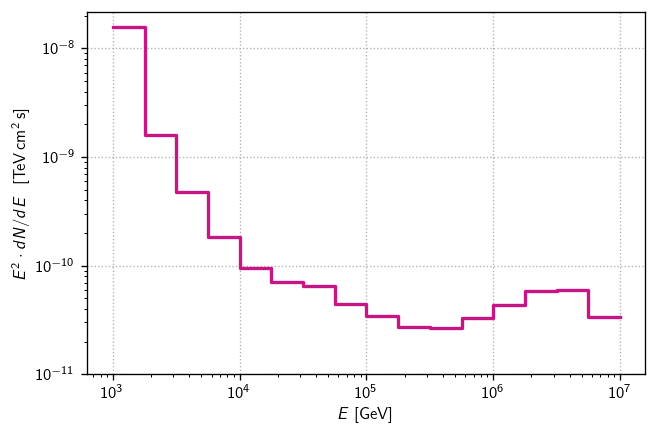
Compared to the original estimates here, these are less optimistic. That seems to be because the final MESC dataset has approximate systematics baked into the signal MC. The impact is significant at lower energies because many events are smeared, and at the highest energies because the per-event smearing is larger.
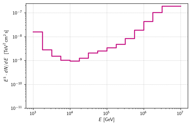
[21]:
fluxs = np.array([s['E2dNdE']/1e3 for s in senss]) # convert GeV->TeV
diffsens3 = hl.Hist(Ebins, (Ebins[:-1]/1e3) * fluxs)
diffsens3
[21]:
Hist(16 bins in [1000.0,10000000.0], with sum 5.887992153145907e-07, 0 empty bins, and 0 non-finite values)
[24]:
fig, ax = plt.subplots()
hl.plot1d(ax, diffsens3, color = color)

ax.loglog()
ax.set(
    ylim=1e-11,
    xlabel=r'$E$ [GeV]',
    ylabel=r'$E^3\cdot dN/dE~~[\text{TeV}^2\,\text{cm}^2\,\text{s}]$',
)
ax.grid()
Note
After computing the differential sensitivity, we tend to show it as a function of the central 90% energy range. The central 90% energy range can be calculated by: 1. Restricting the lower limits of the energy range that is used to inject MC signal events. 2. Compute the sensitivity using this restricted range 3. Repeat until sensitivity changes by 5% 4. Repeat steps 1-3 but restrict the upper limits of the energy range 5. After finding which upper and lower limit cause the sensitivity to change by 5%, we now have the central 90% energy range
[25]:
## Timing summary
print(timer)
ana setup                | 0:00:11.353483
background estimation    | 0:00:11.512436
differential sensitivity | 0:02:28.899687
-----------------------------------------
total                    | 0:02:51.765606
Remarks
Differential sensitivity (or discovery potential) calculations are not very different from energy-integrated ones. The main pitfall is in the n \(\to\) flux conversion. By passing an in-range E0 argument to to_E2dNdE(), we can ensure that the trial runner’s flux instance evaluates to non-zero in that calculation.