Introduction to decision tree classifiers
A decision tree consists of a binary tree with a cut on one variable specified at each node except at the leaf nodes, which have no child nodes. A leaf node may be either a signal leaf or a background leaf. The rest of the nodes may be referred to as split nodes.
An event of unknown class is classified by tracing its path through the tree until a leaf node is reached.
Classification example
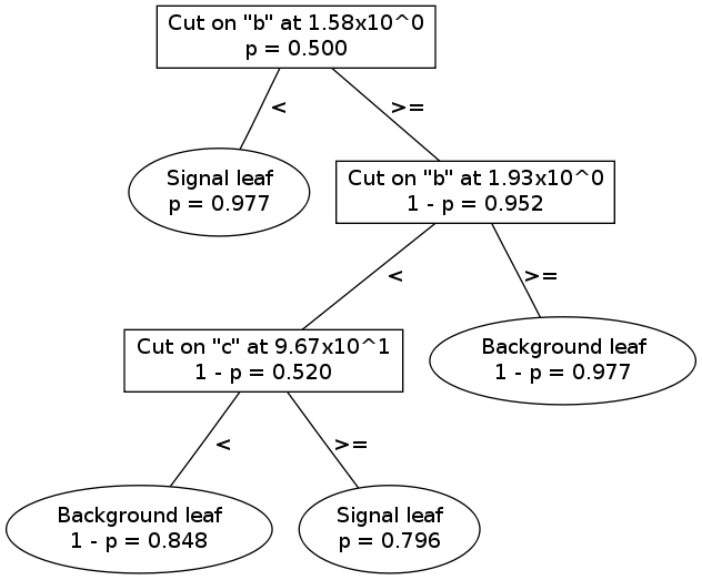
An example is the easiest way to understand how decision trees work. Below is a visualization of the first decision tree from the ABC example.
To see how a single decision tree classifies an event, consider the following sample event:
Variable |
a |
b |
c |
|---|---|---|---|
Value |
2 |
1.7 |
120 |
Using the example decision tree, the event is classified as follows:
At the root node (the one at the top), the cut is at \(b = 1.58\). This event has \(b = 1.7\), so it descends to the right.
At the 2nd node, the cut is at \(b = 1.93\); this event descends to the left.
At the 3rd node, the cut is at \(c = 96.7\); this event descends to the right.
The event lands in a signal leaf.
Thus, on the -1 to +1 scale used by pybdt, this event will be scored +1 by this decision tree.
Some definitions
We can define the following quantities for each node, based on the events in the training example which pass through (for splits) or end up in (for leaves) that node:
- \(w_s\)
The total weight of signal training events in this node.
- \(w_b\)
The total weight of background training events in this node.
- \(W\)
The total weight of training events in this node: \(W=w_s+w_b\).
- \(n_s\)
The number of signal training events in this node.
- \(n_b\)
The number of background training events in this node.
- \(N\)
The total number of training events in this node: \(N=n_s+n_b\).
- \(p\)
The signal purity in this node: \(p = w_s / (w_s + w_b)\). Note that \(1 - p = w_b / (w_s + w_b)\) is the background purity in this node.
We use the following quantities for the \(i\) th event:
- \(x_i\)
The set of cut variable values for the event.
- \(y_i\)
The true identity of an event: +1 for signal events, -1 for background events.
- \(w_i\)
The weight of the event.
- \(s_i\)
The score of the event.
Scoring using purity information
Node purity may be taken as an indicator of signal-like-ness. Assuming that the training samples were representative, an event landing in a higher purity leaf may be more likely to be correctly classified than an event in a lower purity leaf. Thus, there are two ways to score an event: with or without purity information. We may denote a score using purity information as \(s_p\).
In the classification example above, purity information was not used. The example event could only receive a score of either -1 or +1. For a single decision tree, using purity information amounts to calculating a score by simply scaling the leaf node purity: \(s_p = 2p - 1\). Thus, the example event receives a purity score of \(s_p = 0.592\).
Decision tree training
Decision tree training is a recursive process. At a given node, an ensemble of signal training events and background training events remains. Each variable is histogrammed — the number of bins may be chosen by the user — and then the algorithm considers placing a cut at each bin boundary in each histogram. The cut which most increases the signal-background separation is chosen. The training samples are split according to the cut: events on the less-than side go to a new node to the left, and events on the greater-than side go to a new node to the right. The process is repeated recursively for the left and right subsamples. Training continues until a stopping criterion is reached. A leaf is a signal leaf if \(p>1/2\) or a background leaf if \(p<1/2\).
Quantifying cut effectiveness
For each cut variable and value considered, the total weight of signal and background training events which would descend to the left and right, \(W_L\) and \(W_R\) are calculated. Then the child node purities are calculated: \(p_L\) and \(p_R\). Given the purity, a separation criterion may be calculated. Here are the available separation criteria available in pybdt:
- gini (the default)
\(S_G(p) = p\cdot(1-p)\)
- cross entropy
\(S_C(p) = -p\cdot\ln(p) - (1-p)\cdot\ln(1 - p)\)
- misclassification error
\(S_M(p) = 1 - \max (p, 1-p)\)
With the separation criterion specified by the user, the separation gain is calculated for each cut considered: \(\Delta S = W\cdot S(p) - W_L\!\cdot S(p_L) - W_R\!\cdot S(p_R)\). Whichever cut maximizes the separation gain \(\Delta S\) will be selected.
Stopping criteria
Splitting continues until one of the following conditions is reached:
The user-specified maximum depth is reached.
A node has either only signal or only background training events remaining.
The best cut would result in a node with less than the user-specified minimum number of events.