Introduction to boosted decision tree classifiers
A BDT, or boosted decision tree classifier, consists of a forest of decision trees. A user specified number of individual decision trees are trained sequentially, with a boosting process in between each training. Boosting consists of adjusting the weights of individual events according to whether the previously trained tree classifies them correctly. pybdt uses the AdaBoost algorithm for boosting.
The score of an event is a weighted average of the scores the event receives from each tree in the forest.
A BDT may informally be called a “boosted decision tree”, but it must be understood that there are actually many trees (typically hundreds), and that boosting is a process that occurs between the training of consecutive trees.
AdaBoost
After a tree is trained, we can compare the training sample scores \(s_i\) with the training sample true identities \(y_i\). We define a function to indicate whether an event is classified incorrectly: \(I(s,y)=0\) if \(s=y\) and 1 otherwise. Then we calculate the error rate for the tree:
and the boost factor for the tree:
Here, \(\beta\) is a user-specified boost strength (typically between 0 and 1). Once we have the boost factor for the tree, we adjust the weights:
Finally, the weights are renormalized so that \(\sum{}_i w_i = 1\). The new weights are used to train the next tree. After that, the weights are boosted yet again. Boosting is cumulative; the weights are never reset to their original values.
Calculating the BDT score
Consider a set of trees with indices \(m\). The boost factor \(\alpha_m\) calculated during boosting becomes the weight of that tree during scoring. When not using leaf purity information, the score of an event is
However, if the scores are calculated using purity information, the SAMME.R prescription is applied instead. See J. Zhu, H. Zou, S. Rosset, T. Hastie. “Multi-class AdaBoost”, 2009.
Example BDT score distribution
A BDT cannot say definitively whether a given event is a signal or background event. However, most signal events will receive a higher score than most background events. A BDT essentially synthesizes many cut variables with potentially complex relationships into a single, simple cut variable with very good signal/background separation. Here are the score distributions for the BDT in the ABC example:
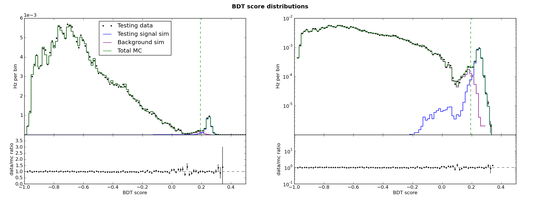
The same information is shown on the left on a linear scale and on the right on a log scale. Note the following features:
The total MC is background-dominated left of about 0.2 and signal dominated right of about 0.2.
Data/MC agreement is quite good, as it must be by construction.
Data/MC agreement is at its worst near the transition from background-dominated to signal-dominated, and at the signal-like tail where very few events remain.
Recall that the background training sample consists of “data” events. In the training data sample, like in the testing data sample, some events are signal like. This is no problem for a BDT, which can tolerate some level of contamination in the training samples. The training algorithm cannot find a way to separate signal-like training background events from training signal events, so it simply never separates them. This is what allows good data/MC agreement even in the signal-like region.