Upgrade and Muon-Bundle Features
In spring 2024, some new features were introduced, in order to allow this project to handle:
Gen-2 and Upgrade DOM’s which will have PMT’s with orientations not necessarily downward.
A primitive model for muon bundles, in which the Cherenkov cone is “truncated”, referred to in the CR-WG as the “Devil’s Tower” model.
The modified wavefront: a truncated Cherenkov cone
Consider this absurdly simple model for a muon bundle: a uniform distribution of muons within some radius (\(R_{bundle}\)), and no muons outside of this radius. The muons are assumed to be moving parallel to each other and aligned in time, so they produce a planewave-like wavefront within this radius, and a Cherenkov-cone wavefront outside of it. Looked at upright, the wavefront looks like a flat-topped mesa – a truncated cone – rather than a pointy-tipped volcano. See these slides from a CR-WG phone call (2023-12-01): https://drive.google.com/file/d/15fVK63UjpsLNhct8FuiTlkCmJTwN7eGP/ for an overview of the motivation for this model (as well as the origin of the name: Devil’s Tower).
This alters the calculation of the geometrical quantities \(t_{geo}\) and \(d_{eff}\) as is described in Algorithms, and it also means that the geometrical calculation is a little different if the DOM is inside the bundle vs. outside of it.
Photon arrival time \(t_{geo}\)
If the DOM is inside the bundle, then the photons arrive at the same time the planewave of muons does: \(t_{\mu} = d_{t}/c\)
If the DOM is outside the bundle, then this is computed exactly as is described in Algorithms, but using a perpendicular distance which is truncated: \(d_{trunc} = d - R_{bundle}\)
Effective distance \(d_{eff}\)
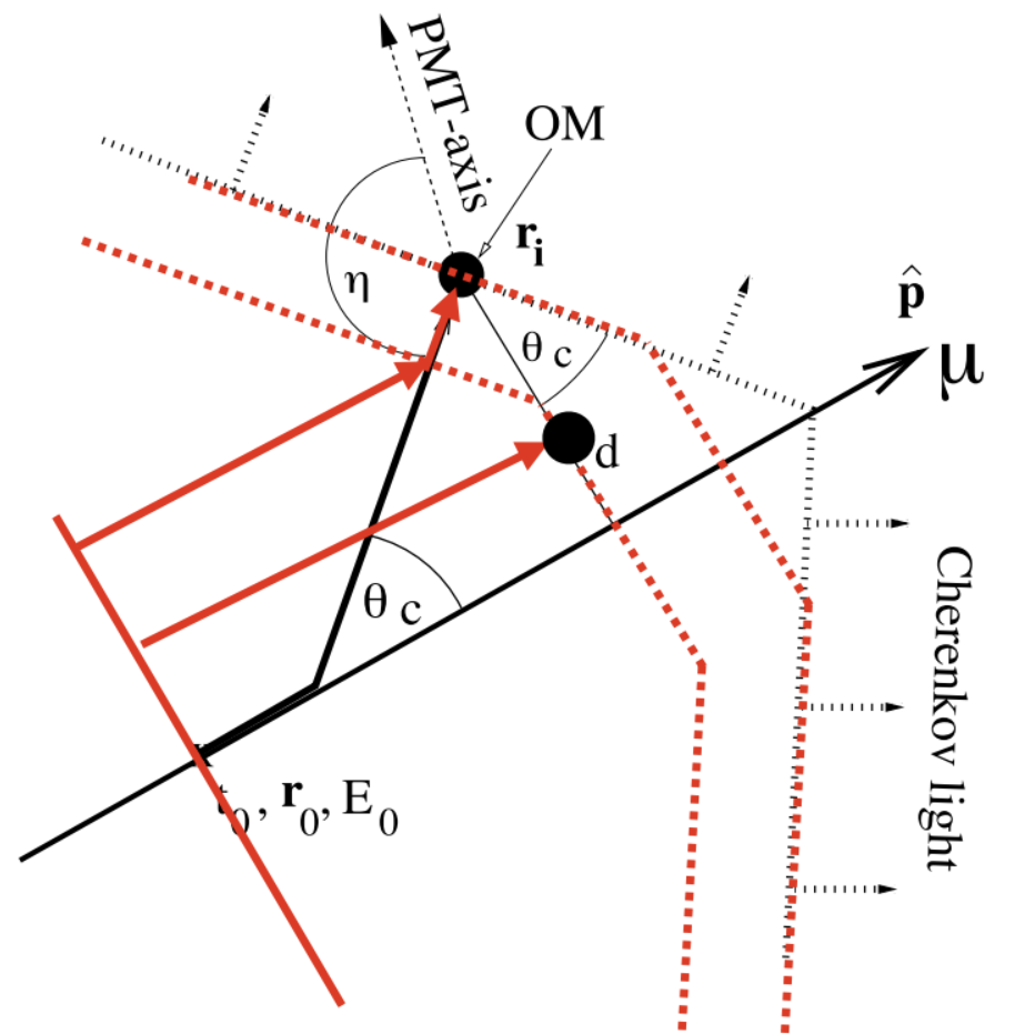
The function for this (described in Algorithms) depends on cos \(\eta\), where \(\eta\) is the angle at which the photons enter the PMT (zero degrees means the photons enter straight in). The calculation of this angle has been overhauled significantly, to account not only for bundle-like hypotheses, but also to account for PMT’s with non-downward orientation (such as in the Upgrade, etc.).
Let’s call the vector direction of the photons’ travel \({\bf \hat p}_{travel}\), and the vector direction of the PMT orientation axis \({\bf \hat n}_{PMT}\). For a standard Gen-1 downward-facing PMT, \({\bf \hat n}_{PMT}\) = (0,0,-1).
In the original code, the photons’ angle of entry was computed simply as \(\cos \eta = {p_{travel}}_z\), assuming that all PMT’s are oriented downward. But if we are to compute this more generally for any PMT, it should be: \(\cos \eta = -{\bf \hat p}_{travel}\cdot{\bf \hat n}_{PMT}\).
If the DOM is inside the bundle, then the photons are traveling in the same direction that the track is. So \({\bf \hat p}_{travel}\) is simply the direction vector of the track, \({\bf \hat p}\).
If the DOM is outside the bundle radius, then the vector direction of travel points from the location along the central track where a Cherenkov photon would depart in order to travel to the DOM, to the position of the DOM:
New arguments for the I3RecoLLH service and its factory
In the original code, \(t_{geo}\) and \(d_{eff}\) were both computed in a function called “muon_geometry”,
located in the source file geometry.cxx.
The updates described here are in a similar but separate function “muon_geometry_bundle”, located in that same file.
Although the function has “bundle” in its name, it can also be used for single-muon hypotheses \((R_{bundle}=0)\)
if you have non-downward-facing PMT’s.
You, the user, can control what method is used in the I3RecoLLH service and its service factory, with these user arguments:
Gen1Fast(boolean): If set to True, this option uses the original “muon_geometry” function instead of “muon_geometry_bundle”; it makes your code backward-compatible with icetray release 1.10.0 or earlier.BundleRadius(float): Radius inside of which to treat the light emission as a planewave. The default value is actually not zero, but a very small number (1e-7 meters), in order to avoid weird floating-point behavior in the calculation of \(d_{eff}\), discussed below.
“BundleRadius” is only relevant if “Gen1Fast” is set to False. The code with throw an error if “BundleRadius” is set to something larger than the default but “Gen1Fast” is also set to True.
Strange things happen very very close to a DOM
The calculation of \(\cos \eta\) uses direction vectors such as \({\bf \hat p}_{travel}\), which are normalized. If a track passes extremely close to a DOM (and we are outside of the bundle), this normalization involves the division of a very small number by another very small number, and strange unstable floating-point behavior can appear. This is true of both the old algorithm and the new one, but differently so, so the results of the two algorithms come out a little different for events where this occurs during the fitting – and it occurs more often than one might think!
If the “inside the bundle” version of \(\cos \eta\) is used, \({\bf \hat p}_{travel}\) comes straight from the track direction and there is not the same division of two very small numbers. Thus, a “minimum bundle radius” is introduced, which kicks in even if the user has not set one by hand (i.e. for a single-muon hypothesis). This radius is very small: 1e-7 meters. So it should not affect Cherenkov times significantly at all. But by giving the hypothesis the “bundle treatment”, the sharp pointy bit of the Cherenkov cone is treated as “rounded off”, by just a little bit. The hope here is to make fits more resistant to strange floating-point effects when the numbers get very small.
The choice of “best” minimum radius, or its effect on fitting, has not been studied extensively. This is a first stab at it.
So, should I use the new algorithm or the old one?
If you are working with Gen-1 events, where all the PMT’s are downward-facing, and you want a normal single-muon hypothesis (not a bundle), then you can set the “Gen1Fast” to either True or False, depending on your taste.
The advantage of “Gen1Fast = True” is that it will run faster. The advantage of “Gen1Fast = False” is that the behavior of the fit should be more robust in cases where a hypothesis track comes extremely close to a DOM, effectively “rounding over the pointy bit of the cone” where mathematical ambiguity lurks. In fact, you as the user could choose where to set the distance at which this “rounding” effect kicks in. (I mean, if a track passes less than a centimeter from a DOM, what does that even mean??) The effect has not been extensively studied as of this writing, but the hope is that it might handle very small numbers better and lead to more sensible results.
If you are working with Upgrade/Gen-2, or another detector where there are PMT’s facing various directions besides downward, you’re going to want to use “Gen1Fast = False”. Otherwise, the \(d_{eff}\)’s will not be computed correctly, which could affect the fit.
And of course, if you want to try a muon-bundle (truncated cone) model rather than a single-muon model, you’ll need to set “Gen1Fast = False” and additionally provide a hypothesis BundleRadius.