Usage
This section currently only covers the standard usage of the module/service chain for IceCube, using a fully parameterized model (i.e. without Geant4).
Basic usage
For a simple simulation run, you should process your I3MCTree using MMC. Then, just use the supplied “tray segment” to add all relevant services and modules to the I3Tray:
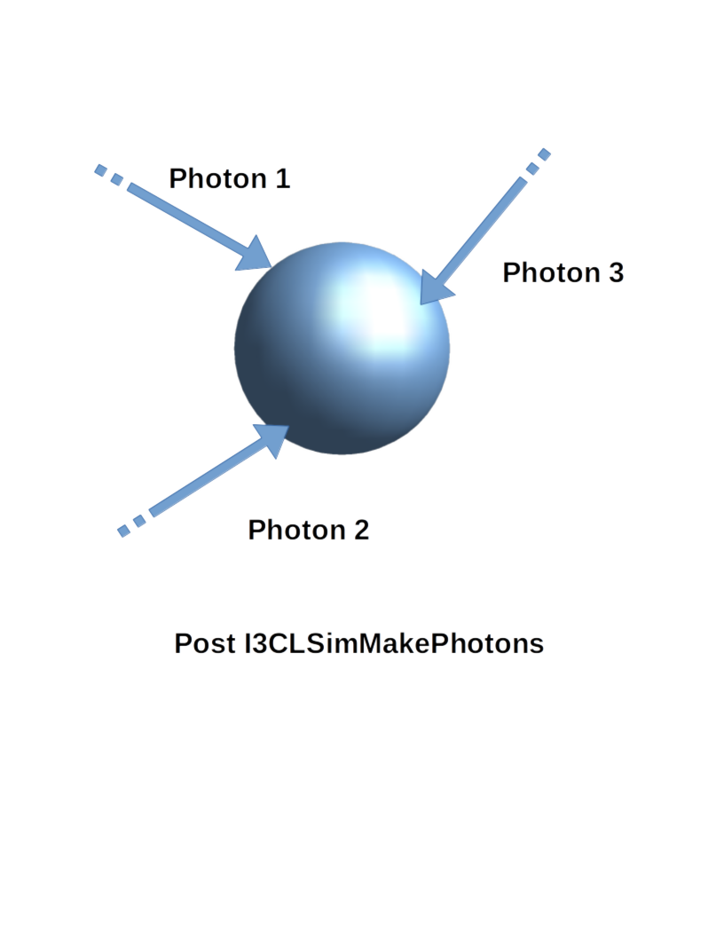
tray.AddSegment(clsim.I3CLSimMakeHits, "makeCLSimHits")
This reads the ‘I3MCTree’ and ‘MMCTrackList’ objects from each frame and adds hits named ‘MCHitSeriesMap’. All photons are generated in a way compatible to ppc.
By default, clsim uses only the GPU for photon propagation (i.e.
CPU devices are skipped during OpenCL device enumeration). This behavior can
be changed using the UseGPUs and UseCPUs boolean options. The following
example would only use the CPU for simulation and skip all GPU devices:
tray.AddSegment(clsim.I3CLSimMakeHits, "makeCLSimHits",
                UseGPUs=False, UseCPUs=True)
Generating Photons using Geant4
By default, clsim does apply photon yield parameterizations compatible to ppc. This can, however, be turned off to use a full Geant4 simulation run. In this case, full GPU simulation might not be necessary because the photon generation will become the bottleneck.
To use Geant4, just enable the UseGeant4 switch:
tray.AddSegment(clsim.I3CLSimMakeHits, "makeCLSimHits",
                UseGeant4=True)
Even in this mode, Geant4 will not be used for muons that have a length
assigned. These are assumed to have been generated by MMC. Both, neutrino-generator
and Corsika generate muons without lengths, so the module should generally
do the right thing. To make absolutely sure that no parameterizations are used,
also set the MMCTrackListName option to None. This will apply Geant4 to all
particles in the I3MCTree (which are InIce and not Dark), even if they
already have a length assigned to them. (You should make sure that this is what you
really want, as MMC might already have added cascades to the muon track that would
be added a second time by Geant4.)
Low-Energy simulations
In order to simulate low energies in a more correct way, you might want to consider disabling the DOM oversizing optimization. It is set to an oversize factor of 5 (in radius), which gives you a 25-fold increase in simulation speed at the expense of accuracy in timing and for tracks very close to DOMs.
To disable DOM oversizing (which might be a good idea especially when using Geant4) use the DOMOversizeFactor switch:
tray.AddSegment(clsim.I3CLSimMakeHits, "makeCLSimHits",
                DOMOversizeFactor=1., # disables oversizing (default is 5.)
                UseGeant4=True)       # enable or disable Geant4 as needed
Ice Models
By default, the ‘SPICE-Mie’ ice model is used. This can, however, easily be changed by supplying either a photonics-compatible ice description file or a ppc-compatible ice description directory using the ‘IceModelLocation’ parameter:
tray.AddSegment(clsim.I3CLSimMakeHits, "makeCLSimHits",
                IceModelLocation=expandvars("$I3_BUILD/clsim/resources/ice/ppc_aha_0.80"))
Another example (using a photonics file) would be:
tray.AddSegment(clsim.I3CLSimMakeHits, "makeCLSimHits",
                IceModelLocation=expandvars("$I3_BUILD/clsim/resources/ice/photonics_wham/Ice_table.wham.i3coords.cos090.11jul2011.txt"))
Example Script
This is a short example script that reads an input .i3 file,
applies MMC and clsim and writes the result to a second file.
It also uses Geant4 for photon generation and is configured to run
on the CPU only. In addition, adding a random number generator using
a python object (instead of a I3Service) is demonstrated.
from icecube.icetray import I3Tray
from os.path import expandvars
import os, sys

from icecube import icetray, dataclasses, dataio, phys_services
from icecube import clsim

I3Seed  = 12345
# a random number generator
randomService = phys_services.I3SPRNGRandomService(
    seed = I3Seed,
    nstreams = 10000,
    streamnum = 1)
tray = I3Tray()

tray.AddModule("I3Reader","reader",
               Filename="input.i3")

tray.AddSegment(clsim.I3CLSimMakeHits, "makeCLSimHits",
    RandomService = randomService,
    UseGPUs=False,
    UseCPUs=True,
    UseGeant4=True,
    IceModelLocation=expandvars("$I3_BUILD/clsim/resources/ice/spice_mie"))

tray.AddModule("I3Writer","writer",
    Filename = "output.i3")

tray.Execute()
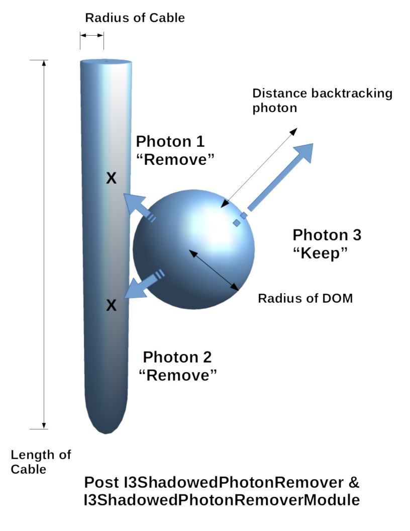
Cable Shadow
While the IceCube DOM has nearly uniform azimuthal acceptance, roughly 1/10th of the photocathode is shadowed by the communications and power cable. The clsim photon propagation kernel accounts for this by recording photon intersections with DOMs only if the photon path does not intersect the cable near the DOM. The cable is assumed to be a vertical, opqaue cylinder with 46 mm diameter and infinite vertical extent, flush with the DOM sphere.
This treatment, however, is disabled by default. It can be enabled by setting
the CableOrientation parameter of I3CLSimMakePhotons (or a derived tray
segment) to the path to a file giving the azimuthal orientation of the cable at
each DOM. Examples include:
ice-models/resources/models/PPCTABLES/cable_position/orientation.led7.txt: positions derived from an analysis of the intensity at neighboring strings when LED 7 was flashed (source-oriented). This assumes that the angle between LED 7 and the cable is always 90 degrees, and constrains the positions to within a few degrees.
ice-models/resources/models/PPCTABLES/cable_position/orientation.shadow.txt: positions derived from an analysis of the received intensity compared to simulation as a function of the simulated cable position. This makes no assumptions on the rotation of the cable w.r.t. to the DOM mainboard, but only constrains the position to tens of degrees.
Either option reduces the average DOM acceptance by 10%, but in a
directionally-specific way. The UnshadowedFraction parameter that has been used
to account for the cable shadow in the past is _not_
automatically adjusted to compensate, so downstream analyzers will have to
handle this themselves. The UnshadowedFraction needs to be set to 1 in this mode.
CUDA propagator
In addition to the OpenCL photon propagation kernel, there is an alternate
implementation in native NVIDIA CUDA, enabled by passing UseCUDA=True to
I3CLSimMakePhotons. This kernel significantly faster than the OpenCL
implementation on 2020-era NVIDIA GPUs, and can run on platforms like POWER9
where NVIDIA does not provide an OpenCL implementation. Details on its
optimization can be found in Hendrik Schwanekamp’s masters thesis.
There are a few operational restrictions to be aware of.
The clsim-cuda library must be compiled against a specific version of the CUDA toolkit (version >= 10). The propagator may fail if it encounters an unsupported GPU driver at runtime.
CMake >= 3.8 is required for CUDA support.
CUDA detection may fail if your C compiler is newer than the CUDA toolkit, e.g. CUDA 10 requires gcc < 8.
Because the kernel is compiled ahead of time, many parameters of the kernel are fixed. The ones that may be set at runtime are:
Absorption and scattering coefficients for 171 ice layers
Photon wavelength distribution
DOM oversize factor
All other parameters will remain at their default values, even if set to another value in the propagator configuration. These include:
The geometry (fixed to IC86)
The form and parameters of the scattering function
ppc interoperability
I3CLSimMakePhotons can also use the propagator from ppc. This makes it
possible to use experimental ice model features directly without first needing
to port them to clsim, as well as comparing implementations of the propagator
using the same input and output stages. To use this, supply a custom setup
function to I3CLSimMakePhotons, e.g.:
from icecube.ppc import MakeCLSimPropagator
tray.AddSegment(clsim.I3CLSimMakePhotons,
   PropagatorSetup=MakeCLSimPropagator,
   ...
)
MakeCLSimPropagator will translate the configuration objects in
DetectorParams into ppc’s preferred configuration format (text files and
environment variables) and return configured instances of
I3LightSourceToStepConverter. Note that since ppc stores its state in
global variables, this converter is a singleton, and you should not use
MakeCLSimPropagator more than once per process.