DOMLauncher
This module simulates the behavior of the DOM mainbaord, including launching and digitization. It reads MCPulses, produced by PMTResponseSimulator, and outputs DOMLaunches. The simulation starts effectively at the anode of the PMT with MCPulses processed by PMTResponseSimulator representing the charge at the anode resulting from a photon hit. This signal is then propagated through the electronics and logics of the DOM to simulate the generation of launches. There are three main features of the DOM that are simulated to generate launches, namely:
Discriminator
Local Coincidence logic
Digitization
Launch decisions based on local coincidence conditions, while being governed by simple rules, generates a complex behavior of the detector. Instead of working out how to handle all different cases based on the entire detector one can model the detector as being built up by objects that follows some rules which make them behave as real DOMs. This model is much simpler since only the communication and the rules have to be implemented.
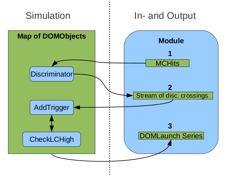
A schematic layout of the flow of data in DOMLauncher. What can be noticed is that the module only handles the IO and the configuration of the DOMObjects, which is not shown in this scheme. MCPulses are processed by the Discriminator() method of the DOMObjects and disc. crossings are put in a global stream. This stream is then fed back to the DOMObjects which then simulate the LC-logic and by the DOMObjects communicating with each other. Once the stream is empty the launches can be gathered from the DOMObjects.
Discriminator
The DOMObjects base their decisions on discriminator threshold crossings. These are simulated with the Discriminator() member function of the DOMObjects. Since the discriminator in a DOM runs independently on the DOM, the discriminator threshold crossings are simulated for each DOMObject for the entire frame. SPE pulse templates, retrieved from calibration, are used together with the MCPulses to model the discriminator waveform. Each time the waveform crosses above a preset threshold it creates a disc. crossing object which is put into the global stream of such crossings. Once all DOMs have had their discriminators simulated the global stream is sorted so it becomes time ordered.
LC-logic
The LC-logic simulation in DOMLauncher depends on the DOMObjects communicating with their neighbors, following the same set of ‘rules’ as the real DOMs and that the DOMTriggers are fed back to the DOMObjects in time order. Most of the ‘rules’ are given in the ICECUBE DOMAPP Firmware Timing Version 0.2 document but restated here in a somewhat different format adapted to the DOMLauncher simulation. The procedure is as follows: when a disc. crossing is received
Check if an LC signal has been sent to the neighbors the last 350 ns.
If true: no action.
If false: Send signals to all connected neighbors.
Launch decision
If busy: throw away the disc. crossing.
If not busy
If no LC signal has been received: Put the disc. crossing in a list of potential launches list
If an LC signal has been received: Check if there are any potential launches from earlier disc. crossing and see if any of them are in i coincidence and decide what kind of launch (SLC, HLC) it will be.
When the DOMObject decides to launch it will not be able to make another launch for some time. i.e it will be busy. The time it is busy depends on the type of launch and the availability of the digitizers. Below follows a table containing the times needed for different operations contributing to the dead time of the DOM and the ATWD chip.
Quantity |
Anotation |
definition |
value |
|---|---|---|---|
ATWD Digitization |
Ad |
The time it takes to digitize one ATWD channel |
29000 [ns] |
ATWD Restart Time |
Ar |
The time it takes to restart the ATWD Chip |
225 [ns] |
ATWD Clear Time |
Ac |
The time it takes to clear one ATWD channel |
950 [ns] |
ATWD Restart Time |
Ar |
The time it takes to restart the ATWD Chip |
225 [ns] |
Cable length corr |
CLr |
The longest time it takes to propagate an LC signal from the furthest neighbor |
1325 [ns] (for in-ice lcspan = 2 regular IceCube DOM) |
Clock Cycle |
Cl |
The length of the FPGA clock cycle |
25 [ns] |
Post window |
Pw |
The length of the FPGA clock cycle |
1000 [ns] (standard icecube) |
The table below shows how the dead time are computed for two kinds of launches and the ATWD chip. Note that there are two ATWD chips on each DOM. Therefore a DOM can have two consecutive HLC launches with the second one starting only 2 clock cycles after the first ended, but a third launch must happen at least 22.5 μ’s
Time busy for |
definition |
value [ns] |
|---|---|---|
SLC Launch |
CLr + Pw + 5 * Cl |
2450 (for in-ice lcspan = 2) |
HLC Launch |
256 fADC samples + 2 * Cl |
6450 |
ATWD Chip Dead Time |
n * Ad + Ar + (4-n)*Ac (n being number of channels to digitize) |
4025 to 116225 |
Digitization
ATWD and fADC digitization is in many ways similar to the discriminator sampling. The difference though is that there is a fixed number of waveform samples to be evaluated, which are digitized and stored, 128 samples for the ATWD and 256 for the fADC. The fADC’s sampling rate is fixed to the FPGA clock cycle while the ATWD has a programmable sampling rate which needs in principle to be checked when simulated, even though the sampling rate has been the same for several years.
The waveform is sampled at the end of each digitizer bin, meaning that if the ATWD starts at time \(t=0\) and the sampling rate corresponds to a bin length 3.3 ns then the first wave form sample is at \(t=3.3\) ns and the next one at \(t=6.6\) ns and so on. All delays affecting the digitizer are applied directly when sampling the waveform. The sample time is given by
where \(t_b\) is the bin time, \(t_h\) is the time of the hit, \(d_t\) the whole transit time including the 75 ns delay line and \(d_d\) is the delta time associated with the different digitizers. When the waveform is first sampled it is temporarily stored as an amplitude in mV with double precision. Then the digitization procedure begins by relating the voltage with digitizer counts still in double precision. Electronic noise is added in counts sampled from a Gaussian distribution centered at 0 with a variance of 0.8 counts for the ATWD. Finally the baseline of the digitizer is added and the counts in double precision are floored and stored as integers. For the ATWD each bin has its unique baseline while the fADC, being a 5 bin long circle buffer, has one nominal baseline for all bins. Furthermore the ATWD digitization returns a true or false depends whether the counts crossed the threshold, of 2/3 (being 768 counts) of the dynamic digitizer range. If the ATWD returns true the digitization of the next ATWD channel with less gain is initiated.
Simulated effects
The following DOM behaviors and physics effects are simulated in DOMLauncher.
Electronic noise in the digitizers
The electronic noise in the digitizers is added on top of the waveform in units of counts. It is modeled by a Gaussian function with a mean = 0 and a variance of 0.8 counts for ATWD digitizers and 0.5 counts for the fADC digitizer. These values are taken from the old DOMsimulator project.
Beacon launches (CPU triggered launches)
Beacon launches are launches that are triggered by the internal CPU onboard the DOM. These launches happen at a constant rate. In real data the rate of beacon launches was 0.6 Hz for data up to the 2014 season and is now 1.2 Hz. Note that a beacon launch is a full readout meaning that all three ATWD channels are read out and 6.4 \(\mu\) s of the fADC read out.
The rate at which beacon launches occur in the simulation can be set with the keyword:
BeaconLaunchRate = 0.6*I3Units.hertz
for the DOMLauncher module. The BeaconLaunch keyword can be set to False to completely omit the simulation of beacon launches.
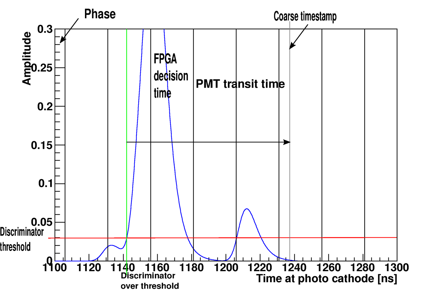
The FPGA Clock phase
Operations performed by the FPGA occur at a discrete times governed by the clock frequency. The FPGA clock frequency is set to 40 MHz which means that the clock cycle length is 25 ns. A DOM launch time will have this granularity of 25 ns. The clock phase between DOMs varies (the global time at which a clock cycle begins for each DOM). Therefore, a random clock phase is added to the clock cycle at each new frame. However, there is also a small drift in the clock cycle, which is not simulated. The effect of the drift should be negligible even for long frames (1 s long). The shifting phase is instead simulated as a RAPcal time uncertainty, which is discussed in the next section.
RAPcal time uncertainty
Optimizations
This section will briefly describe the more complicated optimizations.
Hit Merging
The concept of pulse merging is applied in both DOMLauncher module and PMTResponseSimulator module. A merged pulse is an effective representation of the contributions from single pulses in a time bin. The charge of the merged pulse is the sum of all charge in the bin and the time of the pulse is the charge weighted average time of all pulses in the bin. In PMTResponseSimulator it is applied in a post processing step to reduce memory resources and work load for the subsequent DOMLauncher module using a bin size of 0.2 ns. In the DOMLauncher module a much more aggressive pulse merging is performed using a bin size of 50 ns. However, it is only applied to pulses which are more than 200 ns in the past while evaluating the waveform, “i.e.” pulses which are recovering from droop.
Pulse Template Tabulation
The performance of evaluating pulse templates can be dramatically improved by interpolating the pulse templates. Since the pulse templates are well behaved with three distinct behaviors it was decided to use three linear interpolations with different interpolation steps. To cover the pulse, droop and the initial droop recovery ending at about 100 ns, (depending on the digitizer and channel) a dense interpolation with \(\approx 10\) ps steps is used. During the slower droop recovery up to 6.4 \(\mu\) s a coarser step( around 5 ns) is used.
To account for droop correctly at a given time, the contribution from pulses far in the past must be determined. It was therefore important to interpolate the pulse templates far out in the tails. Since the pulse template falls off exponentially, the derivate has a similar behavior and thus does not change much in the tail. In order to save memory quadratic binning is applied on the interpolation of the pulse template tail.